Prep.Day1

There was no prep for the first day of class. Welcome to Math 214.

Prep.Day2

Task 2.1

Start by looking up the terms vector-valued function and vector parameterization of a curve.

1. Write definitions in your own words for the terms above.
2. For each vector parameterization below, construct a graph of the curve. [Hint: make a table of points if needed, including $t$, $x$, and $y$, and then just plot the $(x,y)$ coordinates).
   1. $\vec r(t) = \left< 2t+1, 4-3t\right>$ for $0\leq t\leq 2$.
   2. $(x,y) = (\cos t, \sin t)$ for $0\leq t\leq 3\pi/2$.
   3. $(x,y)(t) = (\sin t, \cos t)$ for $0\leq t\leq \pi$.
   4. $\langle x,y,z\rangle = (2\cos t, 2\sin t, t)$ for $0\leq t\leq 4\pi$.

Task 2.2

Start by locating a definition of the dot product of two vectors and what it means for two vectors to be orthogonal, as well as the dot product form of the law of cosines.

1. Compute the dot product of the two vectors $\vec a = 3\vec i-4\vec j+2\vec k$ and $\vec b = (-1,3,6)$.
2. Find the angle between $\vec a$ and $\vec b$.
3. Give a value $k$ so that the vectors $\vec a = 3\vec i-4\vec j+2\vec k$ and $\vec c = \langle 2, -1, k\rangle$ are orthogonal.
4. A car is moving in the direction $\vec v = (-5,7)$. The car makes a 90 degree turn to the left. Give a vector that is parallel to this new direction of motion.

Task 2.3

Start by looking up the definition of a unit vector. Consider the two points $P = (1, 2, 3)$ and $Q = (2, −1, 0)$.

1. Write the vector $\vec {PQ} $ in component form $(a, b, c)$.
2. Find the length of vector $\vec {PQ} $.
3. Find a unit vector in the same direction as $\vec {PQ} $.
4. Find a vector of length 7 units that points in the same direction as $\vec {PQ} $.

Task 2.4

The last problem for prep each day will point to relevant problems from OpenStax. Spend 30 minutes working on problems from the sections below.

1. In section 1.1, complete checkpoints 1.1, 1.2, and 1.3. Use the corresponding examples, if needed, to help you.
2. In section 2.3, complete an exercise for each group in 123-144, and then try a few problems in 149-154.

Prep.Day3

Task 3.1

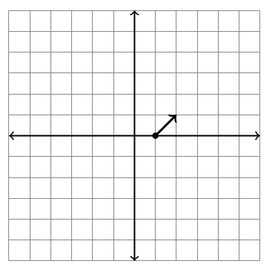
Suppose for a short time that a rover follows a path given by $(x, y) = (1t + 3, −2t + 4)$. This is the same as writing $(x, y) = (1, −2)t + (3, 4)$.

1. Construct a plot that shows the location of the rover at time $t = 0, 1, 2$, and add some arrows as well as a line to illustrate the rover’s path.
2. What is the speed of the rover? (you may assume that distances are in meters, and time is in minutes).
3. What is the rover's velocity (hint, this should be a vector)?
4. When we write the path in the form $(x, y) = (1, −2)t + (3, 4)$, what do the quantities (1, −2) and (3, 4) have to do with the path?
5. The rover is no longer on flat ground, rather is sitting at point $P = (0, 2, 3)$. It starts to climb in the direction $\vec v = \langle 1, −1, 2\rangle$.
   • Write a vector equation $(x, y, z) = (?, ?, ?)$ for the line that passes through the point $P$ and is parallel to $\vec v$.
   • Generalize your work to give an equation of the line that passes through the point $P = (x_1 , y_1 , z_1)$ and is parallel to the vector $\vec v = (v_1 , v_2 , v_3 )$.

Task 3.2

Suppose the Curiosity rover travels in a circular path given by the parametric curve $\vec r(t) = (3 \cos t, 3 \sin t)$.

1. Graph the curve $\vec r$ (you should obtain a circle) and make sure you designate the direction in which the rover is traveling.
2. Compute both $\ds \frac{d \vec r}{dt}$ and $\ds\frac{d^2\vec r}{dt^2}$.
3. Locate the point on your graph that the rover is at when $t = \pi/2$. How would you describe the velocity and acceleration of the rover at this point? Compute both $\frac{d\vec r}{dt}(\frac{\pi}{2})$ and $\frac{d^2\vec r}{dt^2}(\frac{\pi}{2})$, and confirm that these vectors do indeed provide the acceleration and velocity of the rover at $t = \pi/2$.
4. Let's swap to the time $t = \pi/4$. On your graph, draw the vectors $\frac{d\vec r}{dt}(\frac{\pi}{4})$ and $\frac{d^2\vec r}{dt^2}(\frac{\pi}{4})$ with their tail placed on the curve at $\vec r(\frac{\pi}{4})$. These vectors are the velocity and acceleration.
5. Give a vector equation of the tangent line to this curve at $t = \pi/4$.

Task 3.3

Suppose a heavy box needs to be lowered down a ramp. The box exerts a downward force of say 200 Newtons (gravity), which we could write in vector notation as $\vec F=\left<0,-200\right>$. If the ramp was placed so that the box needed to be moved right 6 m, and down 3 m, then we'd need to get from the origin $(0,0)$ to the point $(6,-3)$. This displacement can be written as $\vec d=\left<6,-3\right>$. The force $\vec F$ acts straight down, rather than parallel to the displacement. Let's find out how much of the force $\vec F$ acts in the direction of the displacement. We are going to break the force $\vec F$ into two components, one component in the direction of $\vec d$, and another component orthogonal to $\vec d$. The component of the force that is parallel to $\vec d$ is useful in understanding energy computations. The component of the force that is orthogonal to $\vec d$ is useful in understanding surface friction.

We want to write $\vec F$ as the sum of two vectors $\vec F = \vec w+\vec n$, where $\vec w$ is parallel to $\vec d$ and $\vec n$ is orthogonal to $\vec d$. Since $\vec w$ is parallel to $\vec d$, we can write $\vec w=c\vec d$ for some unknown scalar $c$. This means that $\vec F=c\vec d+\vec n$.

1. Start by drawing a picture that shows how $\vec F$, $\vec d$, $\vec w$, and $\vec n$ are related.
2. Use the fact that $\vec n$ is orthogonal to $\vec d$ to show that $\ds c = \frac{\vec F\cdot \vec d}{\vec d\cdot \vec d}$. [Hint: Dot each side of $\vec F=c\vec d+\vec n$ with $\vec d$ and distribute. You'll need to use the fact that $\vec n$ and $\vec d$ are orthogonal to remove $\vec n\cdot \vec d$ from the problem.]
3. Now that we have a formula for $c$, use that formula to show that $\vec w = c\vec d = (80,-40)$. We call this the projection of $\vec F$ onto $\vec d$ (or the component of $\vec F$ that is parallel to $\vec d$), and write $$\text{proj}_{\vec d}\vec F = \vec F_{\parallel \vec d}= \left(\frac{\vec F\cdot \vec d}{\vec d\cdot \vec d}\right)\vec d.$$
4. Obtain a formula for $\vec n$, the component of the force that is orthogonal to $\vec d$. This is sometimes written as $\vec F_{\perp \vec d}$.

Task 3.4

The last problem for prep each day will point to relevant problems from OpenStax. Spend 30 minutes working on problems from the sections below. Remember that you don't have to do all of the problems listed below, rather do a few from sections that you feel you need more practice with.

• Equations of lines: Section 2.5, checkpoint 2.43 and exercises 243 - 250.
• Derivatives of Vector Valued functions: Section 3.2, checkpoint 3.5 and exercises 41-54.
• Projection practice: section 2.3, checkpoint 2.27 and exercises 167-172

Prep.Day4

Task 4.1

Consider the curve $\vec r(t) = (2t+3, 4(2t-1)^2)$.

1. Construct a graph of $\vec r$ for $0\leq t\leq 2$.
2. If this curve represents the path of a rover (meters for distance, minutes for time), find the velocity of the rover at any time $t$, and then specifically at $t=1$. What is the rover's speed at $t=1$?
3. Give a vector equation of the tangent line to $\vec r$ at $t=1$. Include this on your graph.
4. State the rover's acceleration vector.
5. Explain how to obtain the slope of the tangent line, and then write an equation of the tangent line using point-slope form. [Hint: How can you turn the direction vector, which involves $(dx/dt)$ and $(dy/dt)$, into the number given by the slope $(dy/dx)$?]

Task 4.2

We are ready to tackle the problem of finding the length of a path. This length we call arc length. If a rover moves at a constant speed, then the distance traveled is simply $$\text{distance} = \text{speed}\times\text{time}.$$ This requires that the speed be constant. What if the speed is not constant? Over a really small time interval $dt$, the speed is almost constant, so we can still use the idea above.

Suppose a rover (or other object) moves along the path given by $\vec r(t)=(x(t),y(t))$ for $a\leq t\leq b$. We know that the velocity is $\dfrac{d\vec r}{dt}$, and so the speed is just the magnitude of this vector.

1. Show that we can write the rover's speed at any time $t$ as $$\ds\sqrt{\left(\frac{dx}{dt}\right)^2+\left(\frac{dy}{dt}\right)^2}.$$
2. If the rover moves at speed $\ds\sqrt{\left(\frac{dx}{dt}\right)^2+\left(\frac{dy}{dt}\right)^2}$ for a little time length $dt$, what's the little distance $ds$ that the rover traveled?
3. Explain (Riemann sums may help) why the length of the path given by $\vec r(t)$ for $a\leq t\leq b$ is $$s=\int ds=\int_a^b \left|\frac{d\vec r}{dt}\right| dt=\int_a^b \sqrt{\left(\frac{dx}{dt}\right)^2+\left(\frac{dy}{dt}\right)^2}dt.$$
4. The path $\vec r(t) = (3\cos t, 3\sin t)$ for $0\leq t\leq 2\pi$ is a circle of radius 3. Verify that the formula above does in fact yield the circumference of this circle.
5. If the curve is in space (so $\vec r(t)=(x(t),y(t),z(t))$ is the path), then how does the arc length formula above change?
6. Are there any requirements we must know about the parametrization $\vec r$ so that the formula above is valid?

Task 4.3

Gravity is often the first example we encounter of a vector field. Other important vector fields arise when we study magnetism, electricity, fluid flow, and more. To analyze how a river flows, we can construct a plot of the river and at each point in the river we draw a vector that represents the velocity at that point. This creates a collection of many vectors drawn all at once, where the base of each velocity vector is placed at the point where the velocity occurs. For gravity, a similar picture can be drawn, though all the vectors will point down with the same magnitude. This task has us construct a plot of a vector field.

Consider the function $\vec F(x,y) = \left<x-2y,x+y\right>$. This is a function where the input is a point $(x,y)$ in the plane, and the output is the vector $\left<x-2y,x+y\right>$. For example, if we input the point $(1,0)$, then the output is $\left<1-2(0),1+0\right> = \left<1,1\right>$. To construct a vector field plot, we draw the vector $\left<1,1\right>$ with its base located at the input $(1,0)$. In the picture below, based at $(1,0)$ we draw a vector that points right 1 and up 1.

1. Complete the table below and add the other 7 vectors to the graph.
   \(\begin{array}{c|c} (x,y)&\left<x-2y,x+y\right>\\\hline (1,0)&\left<1,1\right>\\ (1,1)&\\ (1,-1)&\\ (0,1)&\\ (0,-1)&\\ (-1,0)&\\ (-1,1)&\\ (-1,-1)& \end{array}\)
   
2. Repeat the above for the vector field $\vec F(x,y)=(-2y,3x)$, constructing a vector field plot consisting of 8 vectors.

Task 4.4

The last problem for prep each day will point to relevant problems from OpenStax. Spend 30 minutes working on problems from the sections below.

• section 3.2: checkpoint 3.7, exercises 75-92
• Arc Length Practice: section 3.3: checkpoint 3.9, exercises 102-112

Prep.Day5

Task 5.1

Work is a transfer of energy. When a force acts through a displacement, work is done. Gravity acts on falling objects, transferring potential energy to kinetic energy. Any force, when acting through a displacement, will result work done.

• When a constant force and displacement are in the same straight line direction, the work done is simply the product of the magnitude of the force, and the distance.
• When a constant force acts opposite a straight line displacement, the work is the negative of the magnitude of the force and the distance.

If a constant force is not parallel (or antiparallel) to a straight line displacement $\vec d$, then we instead use the component of the force that is parallel to the displacement (so $\vec F_{\parallel \vec d}$) to compute work.

Let $\vec F=(-1,2)$ and $\vec d=(3,4)$.

1. Start by computing $\vec F_{\parallel d} = \text{proj}_{\vec d}\vec F$ and $\vec F_{\perp d}$.
2. Construct a picture that shows the relationship between $\vec F,$ $\vec d$, $\text{proj}_{\vec d}\vec F$, and $\vec F_{\perp d}$.
3. Compute the work done by $\vec F$ through the displacement $\vec d$ by computing $|\vec F_{\parallel d}|$ and $|\vec d|$. Should the work be positive or negative?

Change the force to $\vec F = (-2,0)$. but keep $\vec d=(3,4)$.

4. Construct a similar picture as above, showing the relationship between $\vec F,$ $\vec d$, $\text{proj}_{\vec d}\vec F$, and $\vec F_{\perp d}$. Feel free to construct this picture with, or without, doing any computations.
5. Compute the work done by $\vec F$ through the displacment $\vec d$. Should the work be positive or negative?
6. Can you find a simpler way to compute the work done by $\vec F$ through $\vec d$ than computing $|\vec F_{\parallel d}|$ and $|\vec d|$?

Task 5.2

1. Find the length of the curve $\ds \vec r(t) = \left(t^3,\frac{3t^2}{2}\right)$ for $t\in[1,3]$. The notation $t\in[1,3]$ means $1\leq t\leq 3$. Be prepared to show us your integration steps in class (you'll need a substitution).
2. Now find the length of the helix $\vec r(t) = (2\cos t, 2\sin t, t)$ for $t\in [0, 4\pi] $.

Task 5.3

Suppose a rover is currently moving and has a velocity vector $\vec v = (3,4)$. A force acts on the rover causing an acceleration of $\vec a = (-1,5)$. The rover is currently at the location $(2,-3)$.

1. Draw picture that shows the rover's location along with the velocity and acceleration vectors drawn with their base at the rover's location.
2. Find the vector component of the acceleration that is parallel to the velocity (so find $\vec a_{\parallel \vec v}$), and then find the vector component of the acceleration that is orthogonal to the velocity (so find $\vec a_{\perp \vec v}$).
3. Will this acceleration cause the rover to speed up or slow down? Explain.
4. Will this acceleration cause the rover to turn left or right? Explain.

A probe above Mars is currently moving and has a velocity vector $\vec v = (-2,1,2)$. The onboard thrusters apply a force that causes an acceleration of $\vec a = (0,2,-3)$.

5. Find both $\vec a_{\parallel \vec v}$ and $\vec a_{\perp \vec v}$.
6. Will this acceleration cause the satellite to speed up or slow down? Explain.
7. How would you interpret $\vec a_{\perp \vec v}$?

Task 5.4

The last problem for prep each day will point to relevant problems from OpenStax. Spend 30 minutes working on problems from the sections below.

• Work: section 2.3, checkpoint 2.29 and exercises 175-179
• Projection: section 2.3, checkpoint 2.27 and exercises 167-172
• Arc Length: section 3.3: checkpoint 3.9, exercises 102-112

Prep.Day6

Task 6.1

We can generalize what we've done to find the work done by any force (doesn't have to be constant), acting on any object, along any path. Recall that work is a transfer of energy. Consider the following examples:

• A tornado picks up a couch and applies forces to the couch as it swirls around the center. Work is the transfer of the energy from the tornado to the couch, giving the couch its kinetic energy.
• When an object falls, gravity does work on the object. The work done by gravity converts potential energy to kinetic energy.
• If we consider the flow of water down a river, it is gravity that gives the water its kinetic energy. We can place a hydroelectric dam next to a river to capture a lot of this kinetic energy. Work transfers the kinetic energy of the river to rotational energy of the turbine, which eventually ends up as electrical energy available in our homes.

When we study work, we are really studying how energy is transferred. This is one of the key components of modern life. Recall that the work done by a vector field $\vec F$ through a displacement $\vec d$ is the dot product $\vec F\cdot \vec d$.

• When object moves from $A=(6,0)$ to $B=(0,3)$ encountering the constant force $\vec F = (2,5)$, the work is done by $\vec F$ as the object moves from $A$ to $B$ is simply the displacement $B-A=(-6,3)$ dotted by the force, so we have $W = \vec F\cdot \vec d = (2,5)\cdot(-6,3) = -12+15=3$.

An object moves from $A=(6,0)$ to $B=(0,4)$. A parametrization of the object's path is $\vec r(t) = (-3,2)t+(6,0)$ for $0\leq t\leq 2$.

1. For $0\leq t\leq 1$, the force encountered is $\vec F = (2,5)$. For $1\leq t\leq 2$, the force encountered is $(2,7)$. How much work is done in the first second? How much work is done in the last second? How much total work is done?
2. If we encounter a constant force $\vec F$ over a little displacement $d\vec r$, explain why the little work done is $\ds dW = \vec F\cdot d\vec r =\vec F\cdot \frac{d\vec r}{dt}dt $.
3. Suppose that the force constantly changes as we move along the curve. At $t$, we encountered the force $\vec F(t) = (2,5+2t)$, which we could think of as the wind blowing stronger and stronger to the north. Explain why the total work done by this force along the path is $$\ds W=\int \vec F\cdot d\vec r = \int_0^2 (2,5+2t)\cdot (-3,2)dt.$$ Then compute this integral and show you get 16.
4. If you are familiar with the units of energy, complete the following. What are the units of $\vec F$, $d\vec r$, and $dW$.

If a force of magnitude $F$ acts through a displacement with magnitude $d$, then the most basic definition of work is $W=Fd$, the product of the force and the displacement. Recall that this basic definition has a few assumptions.

• The force $F$ must act in the same direction as the displacement.
• The force $F$ must be constant throughout the displacement.
• The displacement must be in a straight line.

The dot product let's us remove the first assumption as work is $W=\vec F\cdot \vec r,$ where $\vec F$ is a force acting through a displacement $\vec r$. We just saw we can remove the assumption that $\vec F$ is constant to obtain $$W=\int \vec F \cdot d\vec r = \int_a^b F\cdot \frac{d\vec r}{dt}dt, $$ provided we have a parametrization of $\vec r$ with $a\leq t\leq b$. We now get rid of the assumption that $\vec r$ is a straight line.

5. Suppose that we move along the circle $C$ parametrized by $\vec r(t) = (3\cos t,3\sin t)$. As we move along $C$, we encounter a rotational force $\vec F(x,y) = (-2y,2x)$.
   1. Draw $C$. Then at several points on the curve, draw the vector field $\vec F(x,y)$. For example, at the point $(3,0)$ you should have the vector $\vec F(3,0)=(-2(0),2(3))=(0,6)$, a vector sticking straight up 6 units. Are we moving with the vector field, or against the vector field?
   2. Explain why we can state that a little bit of work done by a force $\vec F$ over a small displacement $d\vec r$ is $dW = \vec F\cdot d\vec r$. Why does it not matter that $\vec r$ does not move in a straight line?
   3. Since a little work done by $\vec F$ along $d\vec r$ (a small bit of $C$) is $dW = \vec F\cdot d\vec r$, we know that the total work done is $\int dW = \int \vec F\cdot d\vec r$. This gives us $$W = \int_C\left(-2y,2x\right)\cdot d\vec r = \int_0^{2\pi}\left(-2(3\sin t),2(3\cos t)\right)\cdot(-3\sin t, 3\cos t)dt.$$ Complete the integral, showing that the work done by $\vec F$ along $C$ is $36\pi$.

Task 6.2

Suppose an object travels along the path given by $\vec r(t) = (3t,-2t^2)$. The velocity is $\vec v(t) = (3,-4t)$ and the acceleration is $\vec a(t)=(0,-4)$.

1. Is there a time $t$ at which the velocity and acceleration vectors are parallel? Explain.
2. Compute the vector component of the acceleration vector that is parallel to the velocity vector. In other words, compute $\text{proj}_{\vec v}\vec a$. We'll call this vector $\vec a_{\parallel \vec v}$.
3. What is the vector component of the acceleration vector that is orthogonal to the velocity vector? We'll call this vector $\vec a_{\perp \vec v}$.
4. Draw a picture that shows the relationship among $\vec v$, $\vec a$, $\vec a_{\parallel \vec v}$, and $\vec a_{\perp \vec v}$.

Task 6.3

As the semester goes, we'll be learning to use Mathematica. You can install Mathematica for free as BYU-I student (see here to obtain Mathematica if you do not already have it). If you've never used Mathematica before, no worries. Here is Fast Introduction to Mathematica for Math Students. After reading the "Entering Input" section, feel free to click on the tabs on the left for more information about any topic needed.

1. Let's write a block of code in Mathematica to compute the arc length of any parameterized curve.
   1. First, define a vector function in Mathematica to represent the parameterized curve $\ds \vec r(t) = \left(t^3,\frac{3t^2}{2}\right)$. Something like r = {t^3,3t^2/2}.
   2. Define some variables to hold the upper and lower limits for the parameter $t$ (something like a=1 and b=3).
   3. Add a line to your block of code that uses ParametricPlot[] to create a graph of the function. This verifies that the function is defined correctly.
   4. Compute the derivative or $\vec r$ using the derivative command ( D[]).
   5. Compute the length of the derivative using the Norm[] command.
   6. Compute the arc length of the curve using the Integrate[] command. You can use the N[] command to get a decimal approximation.
   7. Try putting all of the commands above into a single block of code, so that you can run it all with one execution.
2. Copy the block of code that you created, then change the interval of integration to $2\leq t\leq 5$, and see if the plot as well as arc length update.
3. Let's now use the work above to examine arc length for a few other curves. For each curve below, set up an integral formula which would give the length. Then sketch the curve. Try using them in the program you wrote above. Do not worry about integrating them by hand (they will get ugly really fast, and some are impossible).
   1. The parabola $\vec r(t) = (t,t^2)$ for $t\in[0,3]$.
   2. The ellipse $\vec r(t) = (4\cos t,5\sin t)$ for $t\in[0,2\pi]$.
   3. The hyperbola $\vec r(t) = (\tan t,\sec t)$ for $t\in[-\pi/ 4,\pi/4]$.

Task 6.4

The last problem for prep each day will point to relevant problems from OpenStax. Spend 30 minutes working on problems from the sections below.

• Work on paths (line integrals): section 2.3, checkpoint 6.18, example 6.23 and exercises 49-54
• Return to any of the previous day's OpenStax problems to locate extra practice.

Prep.Day7

Task 7.1

Consider the parametric curve $\vec r(t) = (t^2-3t, 4t-5)$ for $0\leq t\leq 3$.

1. Draw the curve.
2. Compute the velocity and speed at any time $t$.
3. Give an equation of tangent line at $t=2$.
4. Compute the acceleration at $t=2$.
5. At $t=2$, compute the vector component of the acceleration that is parallel to the velocity, and the vector component of the acceleration that is orthogonal to the velocity.
6. Set up an integral to compute the arc length of the curve. Then compute the integral (using software is fine).

Task 7.2

Consider the parabolic curve $y=4-x^2$ for $-1\leq x\leq 2$, and the vector field $\vec F(x,y) = (2x+y,-x)$. A parametrization $\vec r(t)$ of this parabolic curve that starts at $(-1,3)$ and ends at $(2,0)$ is $\vec r(t) = (t, 4-t^2)$.

1. Compute $d\vec r$ and state $dx$ and $dy$. What are $M$ and $N$ in terms of $t$?
2. Compute the work done by $\vec F$ on an object that moves along the parabola from $(-1,3)$ to $(2,0)$ (i.e. compute $\int _C Mdx+Ndy$). Check your work using the Sage code at the end of this problem.
3. How much work is done by $\vec F$ to move an object along the same parabola from $(2,0)$ to $(-1,3)$. In other words, if you traverse along a path backwards, how much work is done?
4. We now want to know how much work is done by the same vector field on an object that moves along a straight line from $(-1,3)$ to $(2,0)$.
   • Give a parametrization $\vec r(t)$ of the straight line curve that starts at $(-1,3)$ and ends at $(2,0)$. Make sure you give bounds for $t$.
   • Compute $d\vec r$ and state $dx$ and $dy$. What are $M$ and $N$ in terms of $t$?
   • Compute the work done by $\vec F$ to move an object along the straight line path from $(-1,3)$ to $(2,0)$. Again, check your work using the Sage code at the end of this problem. Note that you must type the times symbol in (3*t-1, ...), otherwise, you'll get an error.
5. Optional (we'll discuss this in class if you don't have it). How much work does it take to go along the closed path that starts at $(2,0)$, follows the parabola $y=4-x^2$ to $(-1,3)$, and then returns to $(2,0)$ along a straight line. Show that this total work is $W=-9$.

var('t','x','y')      #Define your variables
r(t) = (t,4-t^2)      #State your parametrization  
bounds = (t,-1,2)     #Give bounds for the parametrization
F(x,y) = (2*x+y,-x)   #State the vector field
xbounds = (x,-1,2)    #These bounds are useful if you want to make a good plot.
ybounds = (y,0,4)    #These bounds are useful if you want to make a good plot.

dr = r.diff(t)        #Compute the derivative
dW=F(*r(t)).dot_product(dr(t)) #Find a little bit of work.  The code r[0] gives the first component, and r[1] gives the second. 
W=integrate(dW,bounds)

pretty_print(html("""The work done by $F=%s$ along the curve r=$%s$ 
     over the bounds $%s$ is $%s$"""%tuple(map(latex, [F(x,y), r(t), bounds, W]))))
show(table([
[r"$\vec r(t)$", "$(x,y)$", r(t)],
[r"$d\vec r$", "$(dx,dy)$", dr(t)],
["$\vec F(x,y)$", F(x,y), F(*r(t))],
["$M$", F(x,y)[0], F(*r(t))[0]],
["$N$", F(x,y)[1], F(*r(t))[1]],
[r"$dW=\vec F\cdot d\vec r$", "$Mdx+Ndy$", dW],
[r"$W=\int_C \vec F\cdot d\vec r$",W,W]
]
))

p=parametric_plot(r(t),bounds)
p+=plot_vector_field(F,xbounds,ybounds)
show(p)

Task 7.3

Density is generally a mass per unit volume. However, when talking about a wire, it's simpler to let density be the mass per unit length. We can make objects out of composite materials, where the density is different at different places in the object. For example, we might have a straight wire where one end is copper and the other end is gold. In the middle, the wire slowly transitions from being all copper to all gold. Such composite materials are engineered all the time (though probably not our example wire). The density at point $(x,y,z)$ is given by the quantity $\delta (x,y,z)$.

1. Suppose a wire $C$ has the parameterization $\vec r(t)$ for $t\in[a,b]$. Suppose the wire's density (mass per unit length) at a point $(x,y,z)$ on the wire is given by the function $\delta(x,y,z)$. Since density is a mass per length, multiplying density by a small length $ds$ gives us the mass of a small portion of the curve. We represent this symbolically using $dm=\delta(\vec r(t_0)) ds$. Explain why the mass $m$ of the wire is given by the formulas below (explain why each equal sign is true): $$m=\int_C dm = \int_C \delta ds = \int_a^b \delta(\vec r(t)) \left|\frac{d\vec r}{dt}\right|dt.$$
2. Now suppose a wire lies along the straight segment from $(0,2,0)$ to $(1,1,3)$. A parametrization of this line is $\vec r(t) = (t,-t+2,3t)$ for $t\in[0,1]$. The wire's density (mass per unit length) at a point $(x,y,z)$ is $\delta(x,y,z)=x+y+z$.
   1. Is the wire heavier at $(0,2,0)$ or at $(1,1,3)$?
   2. What is the total mass of the wire? [Replace $x$, $y$, $z$, and $ds$ with what they equal in terms of $t$ and then integrate.]
3. Now consider an insulated wire that lies along the curve $\vec r(t) = (7\cos t, 7\sin t)$ for $0\leq t\leq \pi$. The wire contains charged particles where the charge per unit length at location $(x,y)$ is given by $q(x,y)=y$. We'll compute the total charge on the wire.
   1. Draw the curve. Then at several points on the curve write the value of $q(x,y)$ at that point. (Optional: Should the total charge be positive or negative?)
   2. Why is the little charge $dQ$ over a little distance $ds$ approximately given by $dQ = q(x,y)ds$?
   3. The total charge is the sum of the charges over all the little pieces on the rod. This gives us the total charge as $$Q_{\text{total}}=\int_CdQ=\int_C q(x,y)ds = \int_a^b y \sqrt{\left(\frac{dx}{dt}\right)^2+\left(\frac{dy}{dt}\right)^2}dt.$$ Replace $x$ and $y$ with what they are in terms of $t$ and then finish by computing the integral above.

Task 7.4

The last problem for prep each day will point to relevant problems from OpenStax. Spend 30 minutes working on problems from the sections below.

• Return to any of the previous day's OpenStax problems to locate extra practice.

Prep.Day8

Learning Target Checkoff

The first learning target quiz will appear in I-Learn. Complete and submit the quiz before the due date.

Prep.Day9

Task 9.1

We have shown that for a parametric curve given by $\vec r(t)$, for $a\leq t\leq b$, the length of the curve is given by $s = \int_a^b \left|\dfrac{d \vec r}{dt}\right|dt$. We can use a different variable for the parameter, say $\tau$, and then for the curve $\vec r(\tau )$, for $0\leq \tau \leq t$ we get the arc length parameter $$s(t) = \int_0^t \left|\dfrac{d \vec r}{d\tau}\right|d\tau.$$ This provides a function $s(t)$ that tells us the arc length traveled along a curve after $t$ units of time. Note that the derivative of $s(t)$ is (why?) $$\frac{ds}{dt} = \frac{d}{dt}\int_0^t \left|\dfrac{d \vec r}{d\tau}\right|d\tau = \left|\dfrac{d \vec r}{dt}\right|,$$ which is just the speed. By requiring that speed be positive on a curve, then the arc length parameter is an increasing function. This is the reason that the definition of a smooth curve requires that the a parametrization have a nonzero derivative.

1. For the helix $\vec r(t) = (3\cos t, 3\sin t, 4t)$, set up the intergral formula that gives the arc length parameter, and then simplify to show that the arc length parameter is $s(t) = 5t$.
2. If you've traveled 20 units along the helix $\vec r(t) = (3\cos t, 3\sin t, 4t)$, how much time has elapsed? In general, if you've traveled $s$ units, how much time has elapsed. You will have written $t$ as a function of the arc length $s$, obtaining the inverse function $t(s)$.
3. State the functions $\vec r(t)$ and $\vec r(t(s))$. Then compute both $\dfrac{d\vec r}{dt} = \dfrac{d\vec r(t)}{dt}$ and $\dfrac{d\vec r}{ds}=\dfrac{d\vec r(t(s))}{ds}$.
4. Rather than writing $\dfrac{d\vec r}{ds}$ in terms of $s$, it's common to replace $s$ with $s(t)$, giving $\dfrac{d\vec r}{ds}(t)$. Explain why, in general, we have $\dfrac{d\vec r}{ds}(t) = \dfrac{d\vec r/dt}{ds/dt}$.
5. For the curve $\vec r(t) = (a\cos t, a\sin t, bt)$, compute both $\dfrac{d\vec r}{dt}$ and $\dfrac{d\vec r}{ds}$.
6. Show that the magnitude of $\dfrac{d\vec r}{ds}$ is always 1. We call this the unit tangent vector and write $\vec T = \dfrac{d\vec r}{ds}.$

Task 9.2

In this task, we'll show that the product rule applies to the dot product, and then use that to prove that if a vector-valued function has constant length, then the derivative of the function is orthogonal to the original function.

1. Let $\vec r_1(t) = (f(t), g(t))$ and $\vec r_2(t) = (m(t), n(t))$. Prove that $$\frac{d}{dt}(\vec r_1\cdot \vec r_2) = \frac{d}{dt}(\vec r_1)\cdot \vec r_2+\vec r_1\cdot \frac{d}{dt}(\vec r_2).$$
2. Now suppose that $\vec r(t)$ has constant length (meaning $|\vec r(t)|=c$ for some constant $c$). Prove that $\vec r(t) \cdot \dfrac{d\vec r(t)}{dt} = 0$. [Hint, if we know $|\vec r(t)|=c$, what does this mean about $\vec r(t)\cdot \vec r(t)$? How are the dot product and length connected?]
3. Draw the curve $\vec r(t) = (4\cos t+2, 4\sin t-1)$. Show that the velocity has constant length and then verify that the derivative of the velocity (so acceleration) is orthogonal to the velocity.

The problem above gets used quite often in engineering applications. If a beam is attached to a system at a single point, then the beam can rotate about the point. Because the length of the beam is constant, then any rotational forces caused by the beam as it impacts other objects will always be normal to the beam.

Task 9.3

Let $\vec u = (a,b,c)$ and $\vec v = (d,e,f)$. Our goal is to find a single nonzero vector $(x,y,z)$ that is orthogonal to both $\vec u$ and $\vec v$, preferably with as few fractions as possible in the final answer.

1. Explain why we need to solve the system of equations $$ax+by+cz=0\quad\text{and}\quad dx+ey+fz=0.$$
2. To solve the system above, multiply the first equation by $d$ and the second equation by $-a$ (assume for a moment that both $a$ and $d$ are not zero). Then add the two equations together to eliminate $x$, which will allow you to solve for $y$ in terms of $z$. Finish by solving for $x$ in terms of $z$ (there are many ways to do this). You will have shown that every solution to this system can be written in the form $$(x,y,z) = \left(\left(\frac{bf-ce}{ae-bd}\right)z,\left(\frac{cd-af}{ae-bd}\right)z,z\right). $$
3. The above solution has some complicated fractions. Why is $(x,y,z) = (bf-ce, cd-af, ae-bd)$ a solution to the system?

From your work above you will have developed a formula for the cross product of two vectors. The cross product of the two vectors $\vec u = (u_1,u_2,u_3)$ and $\vec v = (v_1,v_2,v_3)$ is the vector $$\vec u\times \vec v = (u_2v_3-u_3v_2, u_3v_1-u_1v_3, u_1v_2-u_2v_1).$$

4. Let $\vec u=(1,-2,3)$ and $\vec v=(2,0,-1)$.
   1. Compute $\vec u\times \vec v$ and $\vec v\times \vec u$. How are they related?
   2. Compute and simplify both $\vec u \cdot (\vec u\times \vec v)$ and $\vec v \cdot (\vec u\times \vec v)$. Did you get zero for both? What fact about the cross product guarantees you get zero?

Task 9.4

The last problem for prep each day will point to relevant problems from OpenStax. Spend 30 minutes working on problems from the sections below.

• Arc Length Parameter: section 3.3: checkpoint 3.10, exercises 127-128, 116, 119, 121, 126
• Look at theorem 3.3 in section 3.2. Properties 4 and 7 were task 9.2. Prove any of the other properties that seem interesting to you.
• Cross product: section 2.4: checkpoint 2.30, exercises 183-192

Prep.Day10

Task 10.1

Given a curve with parametrization $\vec r(t)$, we have already seen that a unit tangent vector is given by $\ds \vec T = \frac{d\vec r}{ds} = \frac{d\vec r/dt}{|d\vec r/dt|}$. Note that this vector has constant length of 1, which means that it's derivative, so $\frac{d\vec T}{dt}$, is orthogonal to $\vec T$. This vector describes how the direction of motion changes. The vector $\ds\vec N = \frac{d\vec T/dt}{|d\vec T/dt|}$ provides a unit vector, we call the principle unit normal vector, that describes the direction in which an object is turning. The cross product $\vec B = \vec T\times \vec N$ we call the binormal vector. These three vectors, namely $\vec T$, $\vec N$, and $\vec B$, provide what we call the Frenet or TNB frame, and are commonly used when describing motion.

1. For the curve $\vec r(t) = (3\cos t, 3\sin t, 4t)$, compute $\vec T$, $\vec N$, and $\vec B$. Show how you obtained each step in your computations.
   • The definitions of $\vec T$ and $\vec N$ both made them one unit long. How long is $\vec B$?
2. For the curve $\vec r(t) = (t,0,t^2)$, compute $\vec T$, $\vec N$, and $\vec B$. Show how you obtained each step in your computations. If things get ugly quite quickly, because of a quotient rule, then you're on the right path.

For a visual representation of the Frenet Frame, please visit this Geogebra site. It's possible to create a very similar visual in Mathematica or Python (something you could aim for with a self-directed learning project).

Task 10.2

Given a parametric curve with parametrization $\vec r(t)$, the curvature vector is the rate of change of the direction of motion with respect to arc length, so $\ds \vec \kappa = \frac{d\vec T}{ds}$. We compute the derivative with respect to arc length so that we obtain a physical property of the curve, rather than a property that relates to how quickly we traverse the curve. The curvature is the magnitude of the curvature vectors, so $$\kappa = |\vec \kappa| = \left| \frac{d\vec T}{ds} \right|.$$ The radius of curvature is the quantity $1/\kappa$.

1. Explain why $\ds \kappa = \frac{|d\vec T/dt|}{|d\vec r/dt|}$.
2. For the circle $\vec r(t) = (5\cos(2t), 5\sin(2t))$, compute the curvature $\kappa$ and radius of curvature $1/\kappa$.
3. For the helix $\vec r(t) = (3\cos(t), 3\sin(t),4t)$, compute the curvature and radius of curvature.
4. For the parabola $\vec r(t) = (t,t^2)$, at $t=0$ compute the curvature $\kappa(0)$ and radius of curvature.
5. Draw the parabola from the previous part. How would you interpret the radius of curvature at $t=0$ in this context?

Task 10.3

Let $P=(a,b,c)$ be a point on a plane in 3D. Let $\vec n=(A,B,C)$ be a normal vector to the plane (so the angle between the plane and $\vec n$ is 90$^\circ$). Let $Q=(x,y,z)$ be another point on the plane.

1. What is the angle between $\vec {PQ} = (x-a,y-b,z-c)$ and $\vec n=(A,B,C)$?
2. Explain why an equation of the plane through $P$ with normal vector $\vec n$ is $$A(x-a)+B(y-b)+C(z-c)=0.$$
3. Consider the three points $R=(1,0,0)$, $S=(2,0,-1)$, and $T=(0,1,3)$. Give an equation of the plane which passes through these three points. [You already have a point on the plane. With three points, you can get two vectors that are in the plane. How can you get a vector that is normal to the plane?]

Task 10.4

The last problem for prep each day will point to relevant problems from OpenStax. Spend 30 minutes working on problems from the sections below.

• Return to any of the previous day's OpenStax problems to locate extra practice.

Prep.Day11

Task 11.1

We'll use Mathematica to create a program to compute all the quantities related to the TNB frame and curvature.

• Download the Mathematica file TNB-intro.nb.
• Read through the introductory examples, evaluating each block of code.
• Adapt the code to compute the TNB frame and curvature for a given curve.

Task 11.2

Recall that the curvature vector is $\kappa = \dfrac{d\vec T}{ds}$, with curvature being a the length of this vector. This vector tells us how much the direction of motion ($\vec T$) changes, as we increase the distance moved along the curve. As such, a tight corner will result in a large change of direction and hence a large curvature. Large corners will result in a small curvature.

The radius of curvature at a point, namely $1/\kappa$, provides the radius of a circle that approximates the shape of curve at that point. Large turns results in a large radius of curvature, while tight turns results in a small radius of curvature. This circle lies in the plane formed by $\vec T$ and $\vec N$ (so a normal vector to this plane is $\vec B$). We call this plane the osculating plane. The center of the circle can be found by following $\vec N$ from the point on the curve.

1. For the curve $\vec r(t) = (3\cos t, 3\sin t, 4t)$, we have already computed $\vec T$, $\vec N$, $\vec B$, and $\kappa$. At $t=\pi/2$, evaluate these quantities.
2. Give an equation of the the osculating plane at $t=\pi/2$. You'll need to identify a normal vector to the plane, and a point on the plane.
3. Explain why the center of curvature is given by $\vec r + \frac{1}{\kappa}\vec N$.
4. Give the location of the center of curvature for $\vec r(t) = (3\cos t, 3\sin t, 4t)$ at $t=\pi/2$.

Task 11.3

There are many ways to compute the TNB frame and curvature. In this problem, we'll develop a few others.

1. Explain why $ \vec N = \dfrac{\vec r^{\prime\prime}_{\perp \vec r^{\prime}}}{ |\vec r^{\prime\prime}_{\perp \vec r^{\prime} }| } $.
2. Explain why $ \vec B = \dfrac{\vec r^{\prime}\times \vec r^{\prime\prime}}{|\vec r^{\prime}\times \vec r^{\prime\prime}|}$.
3. For a function of the form $\vec r(x) = (x, f(x))$, show that $\kappa = \dfrac{|f''(x)|}{(1+(f'(x))^2)^{3/2}}$.

Task 11.4

The last problem for prep each day will point to relevant problems from OpenStax. Spend 30 minutes working on problems from the sections below.

• section 3.3 exercises 113-151

Prep.Day12

Task 12.1

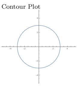
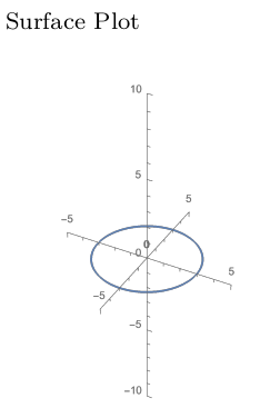
A computer chip has been disconnected from electricity and sitting in cold storage for quite some time. The chip is connected to power, and a few moments later the temperature (in Celsius) at various points $(x,y)$ on the chip is measured. From these measurements, statistics is used to create a temperature function $z=f(x,y)$ to model the temperature at any point on the chip. Suppose that this chip's temperature function is given by the equation $z=f(x,y)=9-x^2-y^2$. (This could just as easily have been the elevation of a rover at a point $(x,y)$ on a hill.) We'll be creating both a 2D contour plot (topographical map) and 3D surface plot of this function in this task.

The points in the plane with temperature $f(x,y)=0$ satisfy $0=9-x^2-y^2$, or equivalently $x^2+y^2=9$. These points lie on a circle of radius 3, so we can draw that circle in the $xy$-plane (the start of our 2D contour plot) and also in 3D by plotting a circle of radius 3 at height $z=0$ (the start of our 3D surface plot). These two plots are shown below.

1. What is the temperature at $(0,0)$, $(1,2)$, and $(-4,3)$?
2. Which points in the plane have temperature $z=5$? Add this contour (level curve) to your 2D contour plot. Then at height $z=5$, add the same curve to the 3D surface plot.
3. Repeat the above for $z=8$, $z=9$, and $z=1$. What's wrong with letting $z=10$?
4. Letting $y = 0$ provides a vertical cross section of the surface. This is the curve $z = 9-x^2-0^2$. This curve cannot be drawn on the contour plot, but can be added to your 3D surface plot. Add that curve, and then add the curve given by letting $x=0$.
5. Describe the 3D surface that you created with your plot. Add any extra features to your 3D surface plot to convey the 3D image you constructed. You can use the Mathematica file ContourSurfaceGradient.nb to check your work.
6. For the function $f(x,y) = x^2-y$, construct a 2D contour plot and 3D surface plot.

Task 12.2

Suppose that an explosion occurs at the origin $(0,0,0)$. Heat from the explosion starts to radiate outwards. Suppose that a few moments after the explosion, the temperature at any point in space is given by $w=T(x,y,z)=100-x^2-y^2-z^2.$

1. Which points in space have a temperature of 99? To answer this, replace $T(x,y,z)$ by $99$ to get $99=100-x^2-y^2-z^2$. Use algebra to simplify this to $x^2+y^2+z^2=1$. Draw this object.
2. Which points in space have a temperature of 96? of 84? Draw the surfaces.
3. What is the temperature at $(3,0,-4)$? Draw the set of points that have this same temperature.
4. The 4 surfaces you drew above are called level surfaces. If you walk along a level surface, what happens to your temperature?
5. When we compute a level surface of a function $w = f(x,y,z)$, which variable do we make constant? When we compute a level curve of a function $z=f(x,y)$, which variable do we make constant?
6. Consider now the function $w=f(x,y,z)=x^2+z^2$. This function has an input $y$, but notice that changing the input $y$ does not change the output of the function.
   • Draw a graph of the level surface $w=4$. [When $y=0$ you can draw one curve. When $y=1$, you draw the same curve. When $y=2$, again you draw the same curve. This kind of graph we call a cylinder, and is important in manufacturing where you extrude an object through a hole.]
   • Graph the level surface $9=x^2+z^2$ (so $w=9$), and $w=16$.

You can use the Mathematica file ContourSurfaceGradient.nb to check your work.

Task 12.3

Suppose the elevation $z$ of terrain near a rover is given by the formula $z=f(x,y) = x^2+3xy$.

1. Suppose that $x$ and $y$ are both functions of $t$, and then use implicit differentiation to compute $\dfrac{dz}{dt}$. Write your answer in the form $$\frac{dz}{dt} = (?)\frac{dx}{dt}+(?)\frac{dy}{dt}.$$
2. The differential of $z$ (or differential of $f$ as $z=f(x,y)$) is obtained by multiplying both sides above by $dt$. Verify that $dz = (2x+3y)dx+3xdy$.
3. Write the differential of $f$ as the dot product $$df = (?,?)\cdot(dx,dy).$$

When we write the differential of a function $f(x,y)$ in the form $df = M dx +N dy$, we call $M$ the partial derivative of $f$ with respect to $x$, written $f_x$ or $\frac{\partial f}{\partial x}$ or $D_x f$, and we call $N$ the partial derivative of $f$ with respect to $y$, written $f_y$ or $\frac{\partial f}{\partial y}$ or $D_y f$. The vector $(f_x,f_y)$ we call the gradient of $f$, written as $\vec\nabla f$, which means the differential of $f$ is always $$df = \vec \nabla f \cdot (dx,dy) = (f_x, f_y)\cdot (dx,dy) = f_xdx+f_ydy.$$ Similar definitions hold for functions of more variables.

4. For the function $f(x,y)=3x^2+2xy$, compute the differential $df$ (in terms of $x$, $y$, $dx$, $dy$), the partial derivatives $f_x$ and $f_y$, and the gradient $\vec \nabla f(x,y)$.
5. For the function $g(r,s,t)=r^2s^3+4rt^2$ compute the differential $dg$ (in terms of $r$, $s$, $t$, $dr$, $ds$, $dt$), the partial derivatives $g_r$ and $\frac{\partial g}{\partial s}$ and $D_tg$, and the gradient $\vec \nabla g(r,s,t)$.

Task 12.4

The last problem for prep each day will point to relevant problems from OpenStax. Spend 30 minutes working on problems from the sections below.

• section 4.1 exercises 14-29, 30-32, 39-41, 42-47, 48-52, 53-58

Prep.Day13

Task 13.1

For the function $f(x,y) = 9-x^2-y^2$, we can compute the differential $df = -2xdx-2ydy$, the partial derivatives $f_x = -2x$ and $f_y=-2y$, along with the gradient $\vec \nabla f(x,y) = (-2x,-2y)$. Notice that the gradient is a vector field, so at the point $(x,y)$ we can draw the vector $(-2x,-2y)$.

1. Construct a plot of the vector field $\vec \nabla f(x,y) = (-2x,-2y)$.
2. Add to your vector field plot a contour plot of $f(x,y) = 9-x^2-y^2$ (we constructed a contour plot for the function in a previous Task).
3. What relationships do you see between the vectors from the gradient plot, and the level curves from your contour plot.

For the function $f(x,y) = x^2-y$, we can compute the differential $df = 2xdx-1dy$, the partial derivatives $f_x = 2x$ and $f_y=-1$, along with the gradient $\vec \nabla f(x,y) = (2x,-1)$. Again, notice that the gradient is a vector field, so at the point $(x,y)$ we can draw the vector $(2x,-1)$.

4. Construct a plot of the vector field $\vec \nabla f(x,y) = (2x,-1)$.
5. Add to your vector field plot a contour plot of $f(x,y) = x^2-y$ (we constructed a contour plot for the function in a previous Task).
6. What relationships do you see between the vectors from the gradient plot, and the level curves from your contour plot.

You can use the Mathematica file ContourSurfaceGradient.nb to check your work.

Task 13.2

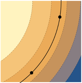
Suppose the Mars rover Curiosity is currently on a hill, and its position is at the center of the map on the left below. Zooming in on the rover's position yields the map on the right below (the color legend applies to the graph on the right).

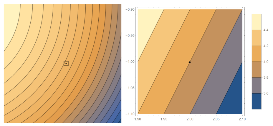
The contours in the graph to the right each represent a change in height of 0.2 units. The bounds for the graph are $1.9\leq x\leq 2.1$ and $-1.1\leq y\leq -0.9$. For simplicity of computations, let's assume the $x$, $y$ and $z$ axes use the same units. The rover is currently located at the point $(2,-1)$, shown as a dot.

The rover can head in many directions. In this problem we'll estimate the slope in several directions. For example, if the rover follows the vector $(0,1)$, heads north, then it has to move a distance (run) of $\Delta y = 0.1$ units to hit the next contour, resulting in a change in height of $\Delta z = +0.2$ units. This means the slope in the $(0,1)$ direction is $$\ds\frac{\text{rise}}{\text{run}} = \frac{\Delta z}{\text{distance moved in $xy$ plane}} = \frac{+0.2}{0.1} = 2.$$

1. Estimate the slope if the rover heads east, following $(1,0)$.
2. If the rover heads south, following $(0,-1)$, estimate the slope.
3. If the rover follows the direction $(1,1)$ (so northeast), what distance must the rover travel to hit the next contour? Use this to estimate the slope in the $(1,1)$ direction.
4. Estimate the slope in the $(1,2)$ direction.

Rather than starting with a contour plot and using it to visually estimate slopes, let's start with a function of the form $z=f(x,y)$ and use it to compute slopes. Suppose the elevation $z$ of terrain near the rover is given by the formula $z=f(x,y) = x^2+3xy$, and the rover is currently at $P=(2,-1)$.

5. Compute the differential $dz$ and write it in the form $dz = (?)dx+(?)dy$. Then evaluate $dz$ at the rover's location $P=(2,-1)$. [Check: Did you get $dz = (1)dx+(6)dy$?]
6. If the rover follows the direction $(dx,dy)$, explain why the slope is $\frac{dz}{\sqrt{(dx)^2+(dy)^2}}$.
7. Estimate the slope if the rover heads east, following $(dx,dy)=(1,0)$. Then estimate the slope if the rover heads north, following $(dx,dy)=(0,1)$. What do these values have to do with the partial derivatives of $f$?
8. Estimate the slope in the $(1,1)$ direction and then the $(1,2)$ direction.

Task 13.3

The volume of a right circular cylinder is $V(r,h)= \pi r^2 h$.

1. If we think of $h$ as a constant, so that $V(r)$ is only a function of $r$, then compute $\frac{dV}{dr}$.
2. If instead we think of $r$ as a constant, so that $V(h)$ is only a function of $h$, then compute $\frac{dV}{dh}$.
3. Compute the differential of $V(r,h)$, and then state the gradient $\vec \nabla V(r,h)$ along with the partial derivatives $\frac{\partial V}{\partial r}$ and $\frac{\partial V}{\partial h}$.
4. If we know $r=3$ and $h=4$, and we know that $r$ could increase by $dr=0.1$ and $h$ could increase by about $dh=0.2$, then use differentials to estimate how much $V$ will increase.

Notice that we were able to compute the partial derivatives above, without ever needing to compute the differential first. We obtain $\frac{\partial V}{\partial r}$ by imagining that every variable other than $r$ was a constant, and then computing the regular derivative.

5. The volume of a box is given by $f(x,y,z)=xyz$. Without computing the differential, compute $\frac{\partial f}{\partial x}$, $\frac{\partial f}{\partial y}$, and $\frac{\partial f}{\partial z}$.
6. Now compute the differential $df$ (use implicit differentiation if needed) and verify that the partial derivatives you computed before actually show up in the differential $df$.
7. If the current measurements are $x=2$, $y=3$, and $z=5$, and we know that expected tolerances are $dx=.01$, $dy=.02$, and $dz=.03$, then estimate the change in volume.

Task 13.4

The last problem for prep each day will point to relevant problems from OpenStax. Spend 30 minutes working on problems from the sections below.

• section 4.3, exercises 118-131

Prep.Day14

We'll spend today revisiting the prep for Day 13. You can jump ahead to day 15 if you want to get ahead. Click to view the Day 13 prep.

Day 13 - Prep

Task 13.1

For the function $f(x,y) = 9-x^2-y^2$, we can compute the differential $df = -2xdx-2ydy$, the partial derivatives $f_x = -2x$ and $f_y=-2y$, along with the gradient $\vec \nabla f(x,y) = (-2x,-2y)$. Notice that the gradient is a vector field, so at the point $(x,y)$ we can draw the vector $(-2x,-2y)$.

1. Construct a plot of the vector field $\vec \nabla f(x,y) = (-2x,-2y)$.
2. Add to your vector field plot a contour plot of $f(x,y) = 9-x^2-y^2$ (we constructed a contour plot for the function in a previous Task).
3. What relationships do you see between the vectors from the gradient plot, and the level curves from your contour plot.

For the function $f(x,y) = x^2-y$, we can compute the differential $df = 2xdx-1dy$, the partial derivatives $f_x = 2x$ and $f_y=-1$, along with the gradient $\vec \nabla f(x,y) = (2x,-1)$. Again, notice that the gradient is a vector field, so at the point $(x,y)$ we can draw the vector $(2x,-1)$.

4. Construct a plot of the vector field $\vec \nabla f(x,y) = (2x,-1)$.
5. Add to your vector field plot a contour plot of $f(x,y) = x^2-y$ (we constructed a contour plot for the function in a previous Task).
6. What relationships do you see between the vectors from the gradient plot, and the level curves from your contour plot.

You can use the Mathematica file ContourSurfaceGradient.nb to check your work.

Task 13.2

Suppose the Mars rover Curiosity is currently on a hill, and its position is at the center of the map on the left below. Zooming in on the rover's position yields the map on the right below (the color legend applies to the graph on the right).

The contours in the graph to the right each represent a change in height of 0.2 units. The bounds for the graph are $1.9\leq x\leq 2.1$ and $-1.1\leq y\leq -0.9$. For simplicity of computations, let's assume the $x$, $y$ and $z$ axes use the same units. The rover is currently located at the point $(2,-1)$, shown as a dot.

The rover can head in many directions. In this problem we'll estimate the slope in several directions. For example, if the rover follows the vector $(0,1)$, heads north, then it has to move a distance (run) of $\Delta y = 0.1$ units to hit the next contour, resulting in a change in height of $\Delta z = +0.2$ units. This means the slope in the $(0,1)$ direction is $$\ds\frac{\text{rise}}{\text{run}} = \frac{\Delta z}{\text{distance moved in $xy$ plane}} = \frac{+0.2}{0.1} = 2.$$

1. Estimate the slope if the rover heads east, following $(1,0)$.
2. If the rover heads south, following $(0,-1)$, estimate the slope.
3. If the rover follows the direction $(1,1)$ (so northeast), what distance must the rover travel to hit the next contour? Use this to estimate the slope in the $(1,1)$ direction.
4. Estimate the slope in the $(1,2)$ direction.

Rather than starting with a contour plot and using it to visually estimate slopes, let's start with a function of the form $z=f(x,y)$ and use it to compute slopes. Suppose the elevation $z$ of terrain near the rover is given by the formula $z=f(x,y) = x^2+3xy$, and the rover is currently at $P=(2,-1)$.

5. Compute the differential $dz$ and write it in the form $dz = (?)dx+(?)dy$. Then evaluate $dz$ at the rover's location $P=(2,-1)$. [Check: Did you get $dz = (1)dx+(6)dy$?]
6. If the rover follows the direction $(dx,dy)$, explain why the slope is $\frac{dz}{\sqrt{(dx)^2+(dy)^2}}$.
7. Estimate the slope if the rover heads east, following $(dx,dy)=(1,0)$. Then estimate the slope if the rover heads north, following $(dx,dy)=(0,1)$. What do these values have to do with the partial derivatives of $f$?
8. Estimate the slope in the $(1,1)$ direction and then the $(1,2)$ direction.

Task 13.3

The volume of a right circular cylinder is $V(r,h)= \pi r^2 h$.

1. If we think of $h$ as a constant, so that $V(r)$ is only a function of $r$, then compute $\frac{dV}{dr}$.
2. If instead we think of $r$ as a constant, so that $V(h)$ is only a function of $h$, then compute $\frac{dV}{dh}$.
3. Compute the differential of $V(r,h)$, and then state the gradient $\vec \nabla V(r,h)$ along with the partial derivatives $\frac{\partial V}{\partial r}$ and $\frac{\partial V}{\partial h}$.
4. If we know $r=3$ and $h=4$, and we know that $r$ could increase by $dr=0.1$ and $h$ could increase by about $dh=0.2$, then use differentials to estimate how much $V$ will increase.

Notice that we were able to compute the partial derivatives above, without ever needing to compute the differential first. We obtain $\frac{\partial V}{\partial r}$ by imagining that every variable other than $r$ was a constant, and then computing the regular derivative.

5. The volume of a box is given by $f(x,y,z)=xyz$. Without computing the differential, compute $\frac{\partial f}{\partial x}$, $\frac{\partial f}{\partial y}$, and $\frac{\partial f}{\partial z}$.
6. Now compute the differential $df$ (use implicit differentiation if needed) and verify that the partial derivatives you computed before actually show up in the differential $df$.
7. If the current measurements are $x=2$, $y=3$, and $z=5$, and we know that expected tolerances are $dx=.01$, $dy=.02$, and $dz=.03$, then estimate the change in volume.

Task 13.4

The last problem for prep each day will point to relevant problems from OpenStax. Spend 30 minutes working on problems from the sections below.

• section 4.3, exercises 118-131

Prep.Day15

Every time we compute a differential $df = f_xdx+ f_ydy$, we're following a pattern that shows up so often that it's given a name (linear combination). At some point you may take a linear algebra course where you'll focus quite a bit on linear combinations, and quickly adopt matrices to help speed up the process of writing linear combinations.

Task 15.1

Let's practice using the definitions above. For each function below, (a) compute and label all relevant partial derivatives. Then (b) write the differential $df$ as a linear combination of the partial derivatives. Then (c) write $df$ as a matrix product. Finish by (d) stating the total derivative $Df$ of the function.

1. $f(x,y)=x^2y$ [Clearly label all 4 things you were asked to find, namely (a) all partials, (b) $df$ as a linear combination, (c) $df$ as a matrix product, and (d) the derivative $Df$.]
2. $f(x,y)=x^2+2xy+3y^2$
3. $f(x,y,z)=3xz-x^2y$

Task 15.2

The gradient of a function $f(x,y)$ is itself a function. When we compute the partial derivatives of the gradient, we obtain vectors instead of numbers. This task has you examine the differential, partials, and derivative of the gradient of a function. We'll soon see that the derivative of the gradient is precisely the key to classifying maximums and minimums of a function.

The function $f(x,y) = x^2+3xy+2y^2$ has the gradient $\vec \nabla f = (2x+3y,3x+4y)$. This is the vector field $$\vec F = (2x+3y,3x+4y).$$

1. Find the differential $d\vec F$ and write it as the linear combination $$d\vec F = \begin{pmatrix}?\\?\end{pmatrix}dx+\begin{pmatrix}?\\?\end{pmatrix}dy.$$
2. Rewrite the above differential as a matrix product, so fill in the blanks below. $$d\vec F = \begin{pmatrix}?&?\\?&?\end{pmatrix}\begin{pmatrix}?\\?\end{pmatrix}.$$
3. Clearly label the two partial derivatives $\frac{\partial \vec F}{\partial x}$ and $\vec F_y$.
4. State the total derivative $D\vec F(x,y)$ (it should be a 2 by 2 matrix). [Note: We also write the derivative of the gradient as $D^2f(x,y)$, or $D\vec\nabla f(x,y)$, and call the resulting matrix the Hessian of $f$. Some people use the notation $\vec \nabla ^2 f$ for the Hessian, though this notation also gets use for the Laplacian $\vec \nabla \cdot (\vec \nabla f)$, which is a very different quantity.]
5. The function $f(x,y) = xy^2$ has gradient $\vec F = (y^2, 2xy)$. Repeat the above to obtain the differential of $\vec F$ (as a linear combination, and in matrix form), the partials of $\vec F$, and the derivative $D\vec F(x,y)$.

Task 15.3

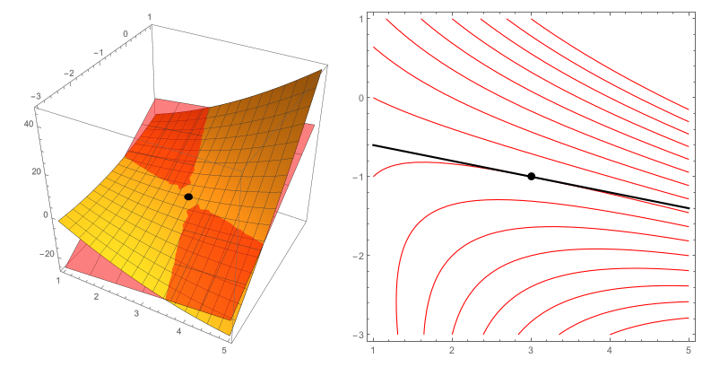
Suppose a rover moves along the level curve of a function $f(x,y)$ following the path $\vec r(t)=(x,y)$. An example of such a scenario is shown below (note that lighter colors correspond to greater outputs of $f(x,y)$. )

Label the dots $A$ and $B$ (it doesn't matter which you label $A$ or $B$). Our goal is to prove that the gradient of $f$ is normal to level curves.

1. At each dot in the picture on the right, draw a vector that represents a possible option for $\ds\frac{d\vec r}{dt} = \left(\frac{dx}{dt},\frac{dy}{dt}\right)$.
2. Suppose $\vec r(0)=A$ and $\vec r(1)=B$. If we know that $f(\vec r(0)) = 7$, then what is $f(\vec r(1))$? Explain.
3. As the rover moves along $\vec r(t)$, how much does $f$ change? Use this to give a value for $\ds\frac{df}{dt}$?
4. Explain why $\vec \nabla f$ and $\ds\frac{d\vec r}{dt}$ are orthogonal at any point along the level curve. (Hint: Add $dt$ to the denominators of the the differential $df = f_xdx+f_ydy$ , and then write the differential as a dot product. Since we are on a level curve, we know the value of $\ds\frac{df}{dt}$.)
5. At point $A$, draw a vector that points in the same direction as $\vec \nabla f(A)$. Use your work above to explain why the gradient of $f$ must be normal to the level curve.

Task 15.4

The last problem for prep each day will point to relevant problems from OpenStax. Spend 30 minutes working on problems from the sections below.

• Return to any of the previous day's OpenStax problems to locate extra practice.

Prep.Day16

Learning Target Checkoff

A learning target quiz will appear in I-Learn. Complete and submit the quiz before the due date.

Prep.Day17

Task 17.1

We'll focus this task on making sure we understand how differentials can help us approximate changes in a function.

A forest ranger needs to estimate the height of a tree. The ranger stands 50 feet from the base of tree and measures the angle of elevation to the top of the tree to be about 60$^\circ$.

1. If this angle of 60$^\circ$ is correct, then what is the height of the tree? Explain in general why the height of the tree is $h(\theta) = 50 \tan \theta$.
2. Compute the differential $dh$ in terms of $\theta$ and $d\theta$.
3. The ranger's angle measurement is mostly likely off by some amount. If the error in the ranger's measurement could be as much as $d\theta = 5^\circ$ (so $\frac{5\pi}{180}$ radians), then use differentials to estimate how large the error in the height could be (so compute $dh$). If your answer here is quite large (much larger than the height of the tree), then look back at your work and see if using radians instead of degrees makes a difference. Why does it? Feel free to ask in class.
4. Compute the height if the angle were exactly 65 instead of 60. What's the actual difference between these two heights?

The US mint creates coins that are roughly a cylindrical shape, with volume $V = \pi r^2h$. Unfortunately, not every coin is exactly the same size, and small errors in $r$ (given by $dr$) and small errors in $h$ (given by $dh$), affect the amount of material needed to mint these coins.

5. Compute $dV$ to give an approximate for the change in volume given by the errors $dr$ and $dh$.
6. The radius of a coin is much larger than the height. Will an error in the radius, or an error in the height, cause a larger change in volume? Explain using your differentials.
7. A soda can company has a cylindrical shape that instead has a large $h$ with small $r$. Will an error in the radius, or an error in the height, cause a larger change in volume in this situation.

Task 17.2

Suppose that our rover is located at point $P=(x,y)$ on a hill whose elevation is given by $z=f(x,y)$. The rover will be moving in the direction parallel to $\vec u$.

1. Explain why the slope of the hill at $P$ in the direction $\vec u = (dx,dy)$ is given by $$\frac{dz}{\sqrt{(dx)^2+(dy)^2}}.$$
2. Prove that this slope can be written, using gradients, as $$\vec \nabla f(P) \cdot \frac{\vec u}{|\vec u|}.$$
3. Use the above fact to compute the slope of a hill given by $f(x,y) = x^2+3xy$ at $P=(2,-1)$ in the direction $\vec u = (3,4)$. (We call this the directional derivative of $f$ at $P$ in the direction $\vec u$, written $D_{\vec u}f(P)$.

The directional derivative of $f$ in the direction of the vector $\vec u$ at a point $P$ is defined to be $$D_{\vec u} f(P)=\vec \nabla f \cdot \frac{\vec u}{|\vec u|}.$$ We can simplify the above to just $f(P)=\vec \nabla f \cdot \hat u$ if $\hat u$ is a unit vector. We dot the gradient of $f$ with a unit vector in the direction of $\vec u$.

4. Show that the partial derivative of $f$ with respect to $x$ is precisely the directional derivative of $f$ in the $(1,0)$ direction.
5. Show that the partial derivative of $f$ with respect to $y$ is precisely the directional derivative of $f$ in the $(0,1)$ direction.

Please watch this short 2 part video that discusses the gradient a bit more, and how you can connect the gradient to the slope in various directions.

• https://www.youtube.com/watch?v=8g2bGLjTLEI&list=PLyLfbaRW-ocMjPvsB_NjXxZDHXSFXUS_A&index=1

Task 17.3

Suppose our rover is located at a point $P$ on a hill whose elevation is given by $z=f(x,y)$. Recall that the directional derivative of $\vec f$ at $P$ in the direction $\vec u$ is the dot product $D_{\vec u} f(P)=\vec \nabla f(P)\cdot \frac{\vec u}{|\vec u|}.$ Also recall that we can compute dot products using the law of cosines $\vec \nabla f(P)\cdot \vec u= |\vec \nabla f(P)| |\vec u|\cos\theta,$ where $\theta$ is the angle between $\vec \nabla f(P)$ and $\vec u$.

1. Give a formula for the angle $\theta$ between the two vectors $\vec \nabla f$ and $\vec u$?
2. Given a direction $\vec u$, the directional derivative will give the slope of $f$ at $P$ in the direction $\vec u$. We want to know which direction we should be pick to obtain the largest slope (directional derivative). Explain why the angle between $\vec u$ and $\vec \nabla f(P)$ must be 0, in order to obtain the largest slope.
3. State a vector $\vec u$ that yields the largest directional derivative.
4. When $\vec u$ is parallel to $\vec \nabla f(P)$, show that $D_{\vec u}f(P) = |\vec \nabla f(P)|$. In other words, explain why the length of the gradient is precisely the slope of $f$ in the direction of greatest increase (the slope in the steepest direction).
5. Which direction points in the direction of greatest decrease? What is the slope in that direction?
6. In your own words, summarize what facts this task helped you learn about the gradient.

Task 17.4

The last problem for prep each day will point to relevant problems from OpenStax. Spend 30 minutes working on problems from the sections below.

• Return to any of the previous day's OpenStax problems to locate extra practice.

Prep.Day18

Task 18.1

In first semester calculus, differential notation is $dy=f' dx$. At $x=c$, the tangent line passes through the point $P=(c,f(c))$. If $Q=(x,y)$ is any other point on the line, then the vector $\vec {PQ} = (x-c,y-f(c))$ tells us that when $dx=x-c$ we have $dy=y-f(c)$. Substitution give us an equation for the tangent line tangent line as $$\underbrace{y-f(c)}_{dy}={f'(c)}\underbrace{(x-c)}_{dx}.$$ This equation tells us that a change in the output ($y-f(c)$) equals the derivative times a change in the input ($x-c$). In this task, we'll repeat this process to obtain an equation of a tangent plane to a function $f(x,y)$, where differential notation gives $$dz = \frac{\partial f}{\partial x}dx+\frac{\partial f}{\partial y}dy.$$

Consider the function $z=f(x,y)=9-x^2-y^2$. We'll be finding an equation of the tangent plane to $f$ at $(x,y)=(2,1)$. Here is surface plot along with the tangent plane at $(2,1,f(2,1))$, together with a contour plot.

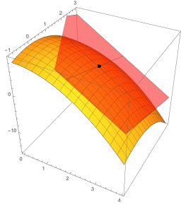
1. Compute the partial derivatives $f_x$ and $f_y$, and the differential $dz$. At the point $(x,y) = (2,1)$, evaluate the partial derivatives and the function $z=f(x,y)$.
2. One point on the tangent plane to the surface at $(2,1)$ is the point $P=(2,1,f(2,1))$. Let $Q=(x,y,z)$ be another point on this plane. Use the vector $\vec{PQ}$ to obtain $dz$ when $dx = x-2$ and $dy = y-1$.
3. We'd like an equation of the tangent plane to $f(x,y)$ when $x=2$ and $y=1$. Differential notation tells us that $$\underbrace{z-?}_{dz}=(-4)\underbrace{(x-?)}_{dx}+(?)\underbrace{(y-?)}_{dy}.$$ Fill in the blanks to get an equation of the tangent plane.
4. Rewrite the equation you got in the form $A(x-a)+B(y-b)+C(z-c)=0$ and state a normal vector to the plane.
5. The level curve of $f$ that passes through $(2,1)$ has no change in height, so $dz=0$. Use this fact to give an equation of the tangent line to this level curve at $(2,1)$.

Now let $z=f(x,y)=x^2+4xy+y^2$. At the point $P=(x,y)=(3,-1)$, we'll give an equation of the tangent plane to the surface and an equation of the tangent line to the level curve of $f$ that passes through this point.

6. Give an equation of the tangent plane at $P=(x,y)=(3,-1)$. [Hint: Find $f_x$, $f_y$, $dx$, $dy$, and then $dz$, all at $(x,y)=(3,-1)$. Then substitute, as done above.]
7. The level curve of $f$ that passes through $P$ is a curve in the plane. Give an equation of the tangent line to this curve at $P$. [Hint: Since we're on a level curve, what does $dz$ equal? The equation is almost identical to the previous part, with one minor change based on what $dz$ equals.]

The tangent plane and tangent line you just found are shown below.

Task 18.2

A rover moves on a hill where elevation is given by $z=f(x,y)=9-x^2-y^2$. The rover's path is parametrized by $\vec r(t)=(2\cos t, 3\sin t)$.

1. At time $t=0$, what is the rover's position $\vec r(0)$, and what is the elevation $f(\vec r(0))$ at that position? Then find the positions and elevations at $t=\pi/2$, $t=\pi$, and $t=3\pi/2$ as well.
2. In the plane, draw the rover's path for $t\in [0,2\pi]$. Then, on the same 2D graph, include a contour plot of the elevation function $f$. Include the level curves that pass through the points in part 1. Along each level curve drawn, state the elevation of the curve. [If you end up with an ellipse and several concentric circles, then you've done this right.]
3. As the rover follows its elliptical path, the elevation is rising and falling. At which $t$ does the elevation reach a maximum? A minimum? Explain, using your graph.
4. As the rover moves past the point at $t=\pi/4$, is the elevation increasing or decreasing? In other words, is $\dfrac{df}{dt}$ positive or negative? Use your graph to explain.

Notice above that we wanted $\frac{df}{dt}$, the rate of change of elevation with respect to time, even though the function $f(x,y)$ does not explicitly have $t$ as an input. The proper notation would be $\frac{d(f\circ r)}{dt}$, but this is so cumbersome that it's generally avoided. The notation $\frac{df}{dt}$ requires the reader to infer from context that $x$ and $y$ depend on $t$.

5. At the point $\vec r(t)$, we'd like a formula for the elevation $f(\vec r(t))$. What is the elevation of the rover at any time $t$? [In $f(x,y)$, replace $x$ and $y$ with what they are in terms of $t$.]
6. Compute $df/dt$ (the derivative as you did in first-semester calculus).

Let's repeat the above, but first compute differentials before substitution. For reference, we let $f(x,y)=9-x^2-y^2$ and $(x,y)=\vec r(t)=(2\cos t, 3\sin t)$.

7. Compute the differential $df$ in terms of $x$, $y$, $dx$, and $dy$.
8. Compute $dx$ and $dy$ in terms of $t$ and $dt$.
9. Use substitution to write $df$ in terms of $t$ and $dt$. Then divide by $dt$ to obtain $\frac{df}{dt}$. Did you get the same answer as the previous part?
10. Use your work above to state both $\vec\nabla f(x,y)$ and $\frac{d\vec r}{dt}$. Show that $\frac{df}{dt} = \vec\nabla f(x,y)\cdot \frac{d\vec r}{dt}$.

Task 18.3

Consider the functions $f(x,y,z) = xy^2z^3$ and $g(x,y)=x\cos(xy)$.

1. First compute $\vec \nabla f$. Then compute $f_{xy}$ and $\frac{\partial^2 f}{\partial z\partial y}$. Explain how you got these. End by computing the entire second derivative $D\vec\nabla f(x,y,z)$ (it is a 3 by 3 matrix with all 9 second partials placed inside).
2. Compute $g_x$ and then $g_{xy}$. Then compute $g_y$ followed by $g_{yx}$.
3. Now let $f(x,y)=3xy^3+e^{x}.$ Compute the four second partials $$\ds \frac{\partial^2 f}{ \partial x^2},\quad \ds\frac{\partial^2 f}{\partial y \partial x},\quad \ds\frac{\partial^2 f}{\partial y^2}, \quad \text{ and }\ds\frac{\partial^2 f}{\partial x \partial y}.$$
4. For $f(x,y)=x^2\sin(y)+y^3$, compute both $f_{xy}$ and $f_{yx}$.
5. Make a conjecture about a relationship between $f_{xy}$ and $f_{yx}$. Then use your conjecture to quickly compute $f_{xy}$ if $$f(x,y)=3xy^2+\tan^{2}(\cos(x)) (x^{49}+x)^{1000}.$$

Task 18.4

The last problem for prep each day will point to relevant problems from OpenStax. Spend 30 minutes working on problems from the sections below.

• Return to any of the previous day's OpenStax problems to locate extra practice.

Prep.Day19

Task 19.1

In the first calculus books, there was no mention of the chain rule. This is because differentials were extremely common notation, and the chain rule, when working with differentials, is simply substitution. In this task, we'll develop some rules for how to compute derivatives when functions depend on other functions (so composite functions).

1. Suppose that $f(x,y,z) = ax+by+cz$, and $x=mt$, $y=nt$, and $z = pt$, for some constants $a,b,c,m,n,p$. Compute the differentials $df$, $dx$, $dy$, and $dz$. Then use substitution to obtain the differential of $f$ in terms of $t$ and $dt$. Finish by stating $\frac{df}{dt}$.
2. Suppose now that $g$ is a function of $x$ and $y$, but $x$ and $y$ are functions of $u$, $v$, and $w$. This means, by definition of the differential and partial derivatives, that $dg = g_xdx+g_ydy$, along with $dx = x_udu+x_vdv+x_wdw$ and $dy = y_udu+y_vdv+y_wdw$. Substitution gives $$\begin{align*} dg &= g_xdx+g_ydy\\ &= g_x(x_udu+x_vdv+x_wdw)+g_y(y_udu+y_vdv+y_wdw)\\ &= (?)du+(?)dv+ (?)dw. \end{align*}$$ Fill in the question marks above, and then use your answer to state the three partials $\dfrac{\partial g}{\partial u}$, $g_v$, and $D_w g$.
3. Consider the function $h(x,y,z)$, where $x$, $y$, and $z$ are functions of $r$ and $\theta$. State the differentials of $h$, $x$, $y$, and $z$, and then use substitution to prove that $$\dfrac{\partial h}{\partial r} = \dfrac{\partial h}{\partial x}\dfrac{\partial x}{\partial r} +\dfrac{\partial h}{\partial y}\dfrac{\partial y}{\partial r} +\dfrac{\partial h}{\partial z}\dfrac{\partial z}{\partial r}.$$ Obtain a similar formula for $\dfrac{\partial h}{\partial \theta}$.

Feel free to ask me in class how this relates to matrix multiplication.

Task 19.2

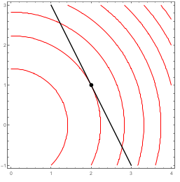
Suppose a rover travels around the circle $g(x,y)=x^2+y^2=1$. The elevation of the surrounding terrain is $f(x,y) = x^2+y+4$. The plot below shows the rover's path (the constraint $g(x,y)=1$), placed on the same grid as a contour plot of the elevation (the function $f(x,y)$ we wish to optimize).

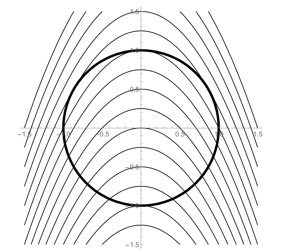
Each level curve above represents a difference in elevation of 0.25 m. Our goal is to find the maximum and minimum elevation reached by the rover as it travels around the circle. We will optimize $f(x,y)$ subject to the constraint $g(x,y)=1$.

1. Label each level curve with its elevation. Print this page, or copy the curves down on your paper.
   • At which $(x,y)$ point does the rover encounter the minimum elevation? What is the minimum elevation? Explain, using the plot.
   • Suppose the rover is currently at the point $(0,1)$ on its circular path. As the rover moves left, will the elevation rise or fall? What if the rover moves right? Is $(0,1)$ the location of a local maximum or local minimum?
   • On your graph, place a dot(s) where the rover reaches a maximum elevation. What is the maximum elevation? Explain.
2. Rather than visually inspecting level curves, let's examine the gradients $\vec \nabla f$ and $\vec \nabla g$ to see how these gradients compare at maximums and minimums.
   • On the graph above, draw $\vec \nabla f$ at lots of places on your contour plot.
   • At lots of points on the circle, with a different color, draw $\vec \nabla g$.
   • Make sure you draw both gradients at all the points corresponding to local maxes and mins.
3. At the local maximums and minimums, Lagrange noticed that $\vec \nabla f = \lambda \vec \nabla g$.
   • How would you interpret the equation $\vec \nabla f = \lambda \vec \nabla g$?
   • Compute $\vec \nabla f$ and $\vec \nabla g$.
   • Explain why the system of equations $\vec \nabla f = \lambda \vec \nabla g$ and $g(x,y)=c$ is equivalent to the system of equations $$2x = \lambda 2x,\quad 1=\lambda 2y,\quad x^2+y^2=1.$$
   • Solve the system of equations above to obtain 4 ordered pairs $(x,y)$. You can use the Mathematica notebook LagrangeMultipliers.nb to check your work.
   • At each ordered pair, find the elevation. What is the maximum elevation obtained, and where does it occur? What is the minimum elevation obtained, and where does it occur?

Task 19.3

This task will mostly involve reading through some definitions and an example, with a short example at the end.

The identity matrix $I$ is a square matrix with 1's on the diagonal and zeros everywhere else, so in 2D we have $I = \begin{pmatrix} 1&0\\0&1 \end{pmatrix}$. To find the eigenvalues, we rewrite $A\vec x = \lambda\vec x$ in the form $A\vec x -\lambda\vec x=\vec 0$ or $A\vec x -\lambda I \vec x=\vec 0$, which becomes $(A-\lambda I) =\vec 0.$ We need to find the values $\lambda$ so that $\left(\begin{bmatrix} a&c\\b&d\end{bmatrix}-\lambda \begin{bmatrix} 1&0\\0&1 \end{bmatrix} \right)\begin{pmatrix}x\\y\end{pmatrix} =\begin{pmatrix}0\\0\end{pmatrix} \quad\text{or}\quad \begin{bmatrix} a-\lambda &c\\b&d-\lambda \end{bmatrix}\begin{pmatrix}x\\y\end{pmatrix} =\begin{pmatrix}0\\0\end{pmatrix}.$ A linear algebra course will show that $\lambda$ satisfies $$(a-\lambda)(d-\lambda)-bc=0.$$

Let's look at an example. Consider $f(x,y)=x^2-2x+xy+y^2$. The gradient is $\vec \nabla f(x,y)=(2x-2+y,x+2y)$. The critical points of $f$ occur where the gradient is zero. We need to solve the system $2x-2+y=0$ and $x+2y=0$, which is equivalent to solving $2x+y=2$ and $x+2y=0$. Double the second equation, and then subtract it from the first to obtain $0x-3y=2$, or $y=-2/3$. The second equation says that $x=-2y$, or that $x=4/3$. So the only critical point is $(4/3,-2/3)$.

The second derivatives is $ D^2f = \begin{bmatrix}2&1 \\1&2\end{bmatrix}.$ The second derivative is constant, so $D^2 f(4/3,-2/3)$ is the same as $D^2f(x,y)$. (In general, the critical point may affect your matrix.) To find the eigenvalues we solve $$(2-\lambda)(2-\lambda)-(1)(1)=0.$$ Expanding the left hand side gives $4-4\lambda + \lambda^2 -1 = 0$. Simplifying and factoring gives us $\lambda^2-4\lambda +3 = (\lambda-3)(\lambda -1) = 0$. The eigenvalues are $\lambda = 1$ and $\lambda=3$. Since both numbers are positive, we know the gradient points outwards away from the critical point. The critical point $(4/3,-2/3)$ corresponds to a local minimum of the function. The local minimum is the output $f(4/3,-2/3) = (4/3)^2-2(4/3)+(4/3)(-2/3)+(-2/3)^2$.

Let's try this process on our own. Consider the function $f(x,y)=x^2+4xy+y^2$.

1. Find the critical points of $f$ by finding when $Df(x,y)$ is the zero matrix.
2. Find the eigenvalues of $D^2f$ at any critical points.
3. Label each critical point as a local maximum, local minimum, or saddle point, and state the value of $f$ at the critical point.

Task 19.4

Pick some problems related to the topics we are discussing from the Text Book Practice page.

Prep.Day20

Task 20.1

Consider the function $f(x,y)=x^3-3x+y^2-4y$.

1. Find the critical points of $f$ by finding when $Df(x,y)$ is the zero matrix.
2. Find the eigenvalues of $D^2f$ at any critical points. [Hint: First compute $D^2f$. Since there are two critical points, evaluate the second derivative at each point to obtain 2 different matrices. Then find the eigenvalues of each matrix.]
3. Label each critical point as a local maximum, local minimum, or saddle point, and state the value of $f$ at the critical point.
4. Use Mathematica to construct a 2D contour plot and 3D surface plot of the function to visually verify that your solution is correct. Choose bounds for your plots so that the critical points are clearly visible.

The Mathematica Notebook 2ndDerTest.nb can help you check much of your work above.

Task 20.2

Let's now return to a Lagrange multiplier problem, where we have a constraint that limits the values over which we want to optimize a function. Consider the curve $xy^2=54$.

1. Start by drawing the curve.

The distance from each point on this curve to the origin is a function that must have a minimum value. We will find a point $(a,b)$ on the curve that is closest to the origin.

The first step to any Lagrange multiplier problem is to identify the function $f(x,y)$ that we wish to maximize or minimize, and then then identify the constraint and write it in the form $g(x,y) = c$. The distance from $(x,y)$ to the origin is $f(x,y) = \sqrt{(x-0)^2+(y-2)^2}=\sqrt{x^2+y^2}.$ This is the function we wish to minimize. The square root on this function will complicate computations later on. Because the square root function is increasing, note that $h(x,y) = x^2+y^2$ will have its minimum value at the same place. Because of this, we can simplify our work and use $f(x,y)=x^2+y^2$ as the function we wish to minimize.

2. What's the constant $c$ and function $g$ so that our constraint can be written in the form $g(x,y)=c$?
3. Solve the system $\vec \nabla f = \lambda \vec \nabla g$ and $g=c$.
   • After computing the gradients, state the 3 equations that form the system we must solve, and then solve it.
   • Note that in this problem, the number $\lambda$ is not an eigenvalue, rather it is a multiplier that helps us know if $\vec \nabla f$ and $\vec \nabla g$ lie on the same line (are parallel or antiparallel, i.e. "Is one gradient a multiple of the other?".
4. State the $(x,y)$ coordinates on the curve $xy^2=54$ that are closest to the origin.

Remember that you can use LagrangeMultipliers.nb to check your work.

5. How does the problem above change if we want to find the point on the curve that is closest to $(3,4)$? Solving the corresponding system of equations by hand will not be simple, but we can use the Mathematica notebook above to quickly answer this question, once we state $f$, $g$, and $c$. You will need to numerically approximate the solution that Mathematica gives (type //N at the end of a line of code to numerically approximate the output). The solution is $(x,y) = (3.11122,4.16612)$.

Task 20.3

Consider the function $f(x,y,z) = -x^2+y^2+z^2$.

1. Start by using the ContourPlot3D[] command in Mathematica to draw several level surface of this function. You can use the Mathematica notebook ContourSurfaceGradient.nb to help you.

The level surface which passes through the point $(3,2,-1)$ is shown below, along with the tangent plane to the surface through the point $(3,2,-1)$. This surface is called a hyperboloid of two sheets.

2. Use the differential $$df = f_xdx+f_ydy+f_zdz \quad\text{or}\quad df=\vec\nabla f(a,b,c)\cdot(dx,dy,dz) . $$ to give an equation of the tangent plane to this surface at the point $(3,2,-1)$. [Hint: Start by explaining why $df=0$. Then we have $dx=x-3$, $dy=y-?$, and $dz =?$. Don't forget to evaluate the partials at the correct point.]
3. Suppose the function $f(x,y,z) = -x^2+y^2+z^2$ gives the temperature (in Celcius) at points in space near some object (located at the origin), with $x,y,z$ values given in meters. Compute the temperature at $(3,2,-1)$, and then use differentials to approximate the temperature at $(3.01,1.98, -0.98)$. [What are $dx$, $dy$, and $dz$?]
4. Compute the directional derivative of $f(x,y,z) = -x^2+y^2+z^2$ at the point $(3,2,-1)$ in the direction $(1, -2, 2)$. What are the units of $D_{ (1, -2, 2) }f(3,2,-1)$?
5. What similarities, and what differences, do you see in the three questions above?

Task 20.4

Pick some problems related to the topics we are discussing from the Text Book Practice page.

Prep.Day21

Task 21.1

Let $f(x,y) = 9-x^2-y^2$. Rather than using Cartesian coordinates to examine this function, we could instead use polar coordinates $x=r\cos \theta$ and $y=r\sin\theta$.

1. Compute the differential $df$ in terms of $x$, $y$, $dx$, and $dy$.
2. Compute the differentials $dx$ and $dy$ in terms of $r$, $\theta$, $dr$, and $d\theta$.
3. Use substitution to obtain $df$ in terms of $r$, $\theta$, $dr$, and $d\theta$. Write your answer as the linear combination $df = (?)dr + (?)d\theta$.
4. State $\frac{\partial f}{\partial r}$ and $\frac{\partial f}{\partial \theta}$.
5. We can write the change of coordinates as the function $(x,y) = \vec T(r,\theta) = (r\cos\theta, r\sin\theta)$. Given a polar coordinate $(r,\theta)$, the function $\vec T$ returns the Cartesian (rectangular) coordinate $(x,y)$. Compute $f(\vec T(r,\theta))$.
6. Compute the differential $d\vec T$ and write is as the linear combination $d\vec T = (?)dr + (?)d\theta$. Note that the questions marks will be vectors, not numbers, because the function $\vec T$ returns a vector (not a number).
7. State the total derivatives $Df(x,y)$ and $D\vec T(r,\theta)$. How would you interpret $Df(\vec T(r,\theta))$.
8. Compute the matrix product $Df(\vec T(r,\theta))D\vec T(r,\theta)$. [Hint: the partial derivatives you computed earlier should appear.]

Task 21.2

This task will have you practice using the second derivative test to locate maxima, minima, and/or saddle points for function $f(x,y)$ of two variables.

1. Consider the function $f(x,y)=x^3-3x+y^2-4y$.
   1. Find the critical points of $f$ by finding when $Df(x,y)$ is the zero matrix.
   2. Find the eigenvalues of $D^2f$ at any critical points. [Hint: First compute $D^2f$. Since there are two critical points, evaluate the second derivative at each point to obtain 2 different matrices. Then find the eigenvalues of each matrix.]
   3. Label each critical point as a local maximum, local minimum, or saddle point, and state the value of $f$ at the critical point.
2. Consider the function $f(x,y) = 6x^2-2x^3+3y^2+6xy$. The function has two critical points $(0,0)$ and $(1,-1)$. At each of these points, evaluate the second derivative and then find the corresponding eigenvalues. Use these eigenvalues to classify each critical point as the location of a local maximum, local minimum, or saddle point.

The Mathematica Notebook 2ndDerTest.nb can help you check much of your work above.

Task 21.3

To use Lagrange Multipliers, we must (1) identify the function $f(x,y)$ to be optimized along with the constant $c$ and function $g$ in the constraint $g(x,y)=c$, (2) write the system of equations that results from $\vec \nabla f = \lambda \vec \nabla g$ and $g(x,y)=c$, (3) solve this system, and (4) determine which points correspond to maxes and which to mins. The third step, solving a system of equations, can become extremely difficult quite quickly, but luckily modern software can help facilitate this part of the process. Please use the Mathematica notebook LagrangeMultipliers.nb to help you check your work and visual what you're doing in this task.

1. Let $f(x,y) = 20 x + 2 y^2$. Use Lagrange multipliers to identify the location of any extreme values of $f$ along the line $100=4x+8y$. Complete this by hand, and then check your work with software.
2. A rover travels along a circle of radius 5, centered at the origin. The elevation of the surrounding hill is give by $z = 4x^2-4xy+y^2$. What are the highest and lowest elevations reached by the rover? [If the system to solve is brutal, then use software to help you.]

Task 21.4

Pick some problems related to the topics we are discussing from the Text Book Practice page.

Prep.Day22

Task 22.1

There are three optimization problems below. Each can be solved with a different method (first semester calculus, Lagrange multipliers, and the second derivative test with eigenvalues). Solve each problem below, and explain your choice of the method used.

1. The elevation near a rover is given by $z=y+x^2$. The rover travels along a path given by $y-2x=5$. Find the $(x,y)$ location of any maxes or mins along the rover's path, and classify the point(s) appropriately.
2. The elevation near a rover is given by $z=y+x^2$. The rover travels along the path parametrized by $\vec r(t) =(t,2t+5)$. Find the $(x,y)$ location of any maxes or mins along the rover's path, and classify the point(s) appropriately.
3. The elevation near a rover is given by $f(x,y)=x^2+xy+y^2-2y$. Determine the location of any maxes or mins near the rover, and classify the point(s) appropriately.

Task 22.2

For each problem below, decide if you'll need to use Lagrange multipliers or the second derivative test. If you choose Lagrange multipliers, then state $f$, $g$, and $c$, along with the system of equations that must be solved. If you choose the second derivative test, then state $f$, $Df$, and $D^2f$. Then use the appropriate Mathematica notebook (either LagrangeMultipliers.nb or 2ndDerTest.nb) to solve the problem.

1. Let $f(x,y)=x^3 + 3xy +y^3$. Find all local extreme values of $f$.
2. Find the dimensions of the rectangle of largest possible area that will fit inside of the ellipse $\frac{x^2}{9}+\frac{y^2}{25}=1$.
3. Find three numbers whose sum is 9 and whose sum of squares is minimized.
4. Find the largest box in the first octant (all variables are positive) that can fit under the paraboloid $z=9-x^2-y^2$. The volume of such a box is given by $V=lwh = xyz = xy(9-x^2-y^2)$.
5. A rover travels along a circle of radius 5, centered at the origin. The elevation of the surrounding hill is give by $z = 4x^2-4xy+y^2$. What are the highest and lowest elevations reached by the rover.

Task 22.3

In this task we'll derive the version of the second derivative test that is found in most multivariate calculus texts. The test given below only works for functions of the form $f:\mathbb{R}^2\to\mathbb{R}$. The eigenvalue test you have been practicing will work with a function of the form $f:\mathbb{R}^n\to\mathbb{R}$, for any natural number $n$.

Suppose that $f(x,y)$ has a critical point at $(a,b)$.

1. We know that $D^2f(a,b) = \begin{bmatrix}f_{xx}&f_{xy}\\f_{yx}&f_{yy}\end{bmatrix}$, where all partials are evaluated at $(a,b)$. Prove that the eigenvalues of $D^2f(a,b)$ are given by $$\lambda = \frac{(f_{xx}+f_{yy})\pm \sqrt{(f_{xx}+f_{yy})^2 - 4(f_{xx}f_{yy}-f_{xy}^2)}}{2}.$$
2. Let $D=f_{xx}f_{yy}-f_{xy}^2$.
   1. If $D<0$, explain why the eigenvalues differ in sign.
   2. If $D=0$, explain why zero is an eigenvalue.
   3. If $D>0$, explain why the eigenvalues must have the same sign.
   4. If $D>0$, and $f_{xx}>0$, explain why $f$ has a local minimum at $(a,b)$.
   5. If $D>0$, and $f_{xx}<0$, explain why $f$ has a local maximum at $(a,b)$.
   6. How would you interpret $f_{xx}$ in terms of concavity?
3. The only critical point of $f(x,y) = x^2+3xy+2y^2$ is at $(0,0)$. Does this point correspond to a local maximum, local minimum, or saddle point? Find $D$ from part 2 to answer the question.

Task 22.4

Pick some problems related to the topics we are discussing from the Text Book Practice page.

Prep.Day23

We won't have any new tasks today, rather we'll focus on finishing up any tasks we have not yet discussed in class from prior days.

Prep.Day24

Learning Target Checkoff

A learning target quiz will appear in I-Learn. Complete and submit the quiz before the due date.

Prep.Day25

We are beginning a new unit on integration.

Task 25.1

We need to become adept at describing regions in the plane, using inequalities. For this first task, we'll start with inequalities and from them shade a region in the plane.

1. Shade the region in the $xy$-plane that satisfies the inequalities $-1\leq x\leq 1$ and $1-x\leq y\leq 4-x^2$.
2. Shade the region in the $xy$-plane that satisfies the inequalities $-3\leq y\leq 0$ and $0\leq x\leq \sqrt{9-y^2}$.
3. Shade the region in the $xy$-plane that satisfies the polar coordinate inequalities $0\leq \theta\leq \pi$ and $1\leq r\leq 3$.
4. Shade the region in the $xy$-plane that satisfies the polar coordinate inequalities $-\frac{\pi}{6}\leq \theta \leq \frac{\pi}{6}$ and $0\leq r\leq 4\cos 3\theta$.
5. Shade the region in the $xy$-plane that satisfies the polar coordinate inequalities $0\leq \theta\leq \frac{3\pi}{2}$ and $1\leq r\leq 3+2\cos\theta$.

We can also describe solid regions in space, using 3 sets of inequalities.

6. Draw the region in space that satisfies the inequalities $0\leq x\leq 3$, $-1\leq y\leq 1$, and $0\leq z\leq 1-y^2$.
7. Draw the region in space that satisfies the inequalities $-1\leq x\leq 1$, $0\leq y\leq 1-x^2$, and $0\leq z\leq 1-y$.

Task 25.2

One way to compute the area of a region $R$ is overlay the region with a rectangular grid, where $dx$ and $dy$ are the distances between the vertical and horizontal lines of the grid. To find the area of the region, we first determine which of the rectangles contains a portion of the region $R$, and then add up the areas of of all such rectangles. This will overestimate the area, but we can then use limits to shrink both $dx$ and $dy$ to zero to obtain the area.

Consider the polar curve $r=1+\cos\theta$. We will use the approach described above to estimate the area of region $R$ that is inside this polar curve. We'll assume that all distances are given in meters. The bounds for each graph below are $-1\leq x\leq 2$ and $-2\leq y\leq 2$.

1. For the first picture above, there are 10 rectangles (shaded) that contain a portion of the region $R$. Each of these rectangles has area $dA=dxdy=(1)(1) = 1 $, which means an overestimate for the area of $R$ is $A\approx 10 \, dA = 10(1)=10$. Describe a way to use these same rectangles to get an underestimate for the area of $R$.
2. Now use the middle picture above (where $dx=dy=.5$) to shade and then count the number of rectangles that contain a portion of $R$. What is the area $dA$ of each little rectangle. Finish by giving an estimate for $A$.
3. Now use the last picture with $dx=dy=.2$ to estimate the area of $R$.
4. How can we obtain the exact value for the area of $R$?
5. The questions above help focus on finding area, because each rectangle was given the same importance in the overall sum. Suppose instead that an object is made in the shape of the cardioid, but the portion that lies above the $x$-axis has a density of 2 kg/m^2, while the portion below has a density of 3 kg/m^2. How would you modify your work above to give an estimate for the mass (in kg)?

Task 25.3

In this task, we'll focus on the integrals $\int_C dx$ and $\int_C dy$, and from them develop a way to compute area using iterated (repeated) integrals.

1. Consider the portion of the ellipse parametrized by $\vec r(t) = (3\cos t, 4\sin t)$ for $0\leq t\leq \pi/2$. Notice that parametrization starts at $(3,0)$ and ends at $(0,4)$. The integral $\int_C dx$ literally says ``Sum up little changes in $x$.'' Adding up little changes in $x$ gives the total change in $x$.
   • Differentials gives us $dx = -3\sin t dt$. Compute $\ds\int_C dx=\int_{t=0}^{t=\pi/2}dx = \ds\int_{t=0}^{t=\pi/2}-3\sin t dt$ and verify that it gives the total change in $x$ from $t=0$ to $t=\pi/2$.
   • Guess the value of $\ds\int_{t=0}^{t=\pi/2}dy$ (the integral adds up what?), and then check your solution.
2. Consider the region $R$ between the functions $y=x^2$ and $y=-x$ for $0\leq x\leq 3$. Our goal is to explain why the iterated integral $\ds\int_{x=0}^{x=3}\left(\int_{y=-x}^{y=x^2} dy \right)dx$ gives the area of the region $R$.
   • Draw both functions and shade the region $R$.
   • Compute the integral $\ds\int_{y=-x}^{y=x^2}dy$ for arbitrary $x$. This integral comutes, for a given value of $x$, the total change in $y$ (so a height).
   • Recall that $dx$ is a small width. When we multiply the previous integral by this width $dx$, we will obtain the area of a small rectangular region whose height is given by $\ds\int_{y=-x}^{y=x^2}dy$ and width is given by $dx$. Pick a value $x$ between 0 and 3, and then construct a picture that illustrates this rectangular region whose area is given by $dA=\ds\left(\int_{y=-x}^{y=x^2} dy \right)dx$.
   • Explain why $\ds\int_{x=0}^{x=3}\left(\int_{y=-x}^{y=x^2} dy \right)dx$ gives the area of the region $R$.
3. Consider the double integral $$\int_{y=-1}^{y=2}\left(\int_{x=y^2}^{x=y+2}dx\right)dy.$$
   • The bounds in the integral above describe a region in $xy$ plane where $-1\leq y\leq 2$ and $y^2\leq x\leq y+2$. Sketch this region.
   • Consider the inner integral $\int_{x=y^2}^{x=y+2}dx$. This integral adds up changes in $x$, so gives a total change in $x$ (hence a width). Add to your sketch several line segments whose widths are given by this integral.
   • When we multiply a width $\int_{x=y^2}^{x=y+2}dx$ by a small height $dy$, we get a little bit of area $dA$. Pick a value $y$ between $-1$ and $2$, and then at that height draw a small rectangle whose area is given by $dA = \left(\int_{x=y^2}^{x=y+2}dx\right) dy$.
   • Adding up little bits of area gives total area, so the double integral $$\int_{y=-1}^{y=2}\left(\int_{x=y^2}^{x=y+2}dx\right)dy$$ gives an area. Compute the integral.

Task 25.4

Pick some problems related to the topics we are discussing from the Text Book Practice page.

Prep.Day26

Task 26.1

In this task we'll be focusing on locating the average, mean, center, etc., of something.

1. Suppose a class takes a test and there are three scores of 70, five scores of 85, one score of 90, and two scores of 95. We will calculate the average class score, $\bar s$, four different ways to emphasize four ways of thinking about the averages. We are emphasizing the pattern of the calculations in this problem, rather than the final answer, so it is important to write out each calculation completely, without doing any simplifying, before calculating the number $\bar s$.
   1. Compute the average by adding 11 numbers together and dividing by the number of scores ($\bar s=\frac{\sum \text{values}}{\text{number of values}}$). Write down the whole computation before doing any arithmetic.
   2. Compute the numerator of the fraction in the previous part by multiplying each score by how many times it occurs, rather than adding it in the sum that many times ($\bar s=\frac{\sum (\text{value}\cdot\text{weight})}{\sum \text{weight}}$). Again, write down the calculation for $\bar s$ before doing any arithmetic.
   3. Compute $\bar s$ by splitting up the fraction in the previous part into the sum of four numbers ($\bar s=\sum (\text{value}\cdot\text{(\% of stuff)})$). This is called a weighted average because we are multiplying each score value by a weight.
   4. Another way of thinking about the average $\bar s$ is that $\bar s$ is the number so that if all 11 scores were the same value $\bar s$, you'd have the same sum of scores ($\text{ (number of values) }\bar s = \sum \text{values}$ or $(\sum \text{weight})\bar s = \sum (\text{value}\cdot\text{weight})$). Write this way of thinking about these computations by taking the formulas for $\bar s$ in the first two parts and multiplying both sides by the denominator.

We now generalize the above ways of thinking about averages from a discrete situation to a continuous situation. We did this in first-semester calculus when we computed the average value of $f$ using integrals.

2. Suppose the price of a stock is \$10 for two days. Then the price of the stock jumps to \$20 for three days. Our goal is to determine the average price of the stock over the total 5 day period.
   1. Why is the average stock price not \$15? Use any of the methods from the previous problem to show that the average price is $\bar f=\$16$.
   2. The function $f(t) = \begin{cases}10 &0\leq t<2\\20&2\leq t\leq 5\end{cases}$ models the price of the stock for the 5-day period. The graph below shows both the function $f$ and the average stock price $\bar f$. Show that the area under $f$ for $0\leq t\leq 5$ is 80. Then show that the area under $\bar f$ for $0\leq t\leq 5$ is also 80.
      
   3. The average value of a function over an interval $ [a,b] $ is a constant value $\bar f$ so that the areas under both $f$ and $\bar f$ are equal, which means $\ds\int_a^b \bar f dx = \int_a^b f dx.$ Solve for $\bar f$ to show that $$\bar f = \dfrac{\ds\int_a^b f dx}{\ds\int_a^b dx}.$$

Let's examine one last averaging question, this time as it relates to a rover. If we know the mass and center-of-mass of each part of the rover, we can use weighted averages to combine these values and obtain the center-of-mass of the the entire rover.

3. Consider a simplified rover with a bottom and a top.

• The bottom part of the rover has a volume of $V_1$ m$^3$, a constant density (mass per volume) of $\delta_1$ g/m$^3$, and a center-of-mass located at $(\bar x_1,\bar y_1,\bar z_1)$.
• The top part of the rover has a volume of $V_2$ m$^3$, a constant density (mass per volume) of $\delta_2$ g/m$^3$, and a center-of-mass located at $(\bar x_2,\bar y_2,\bar z_2)$.
  1. Give the masses $m_1$ and $m_2$ of the bottom and top of the rover. Explain.
  2. What proportion of the total mass comes from the bottom of the rover?
  3. Explain why the center-of-mass of the entire rover is $$\left(\frac{\bar x_1(m_1)+\bar x_2(m_2)}{m_1+m_2},\frac{\bar y_1(m_1)+\bar y_2(m_2)}{m_1+m_2}, \frac{\bar z_1(m_1)+\bar z_2(m_2)}{m_1+m_2}\right) .$$
  4. The rover picks up an additional object. The object's mass is $m_3$ with center-of-mass $(\bar x_3, \bar y_3, \bar z_3)$. Modify the formula above to give the center-of-mass of the rover, together with the new object. Try writing the formula using summation notation.

Task 26.2

To find the mass of a thin metal plate occupying a region $R$ in the $xy$-plane, we add up the little masses (differentials) $dm = \delta(x,y)dA$, where $\delta$ is the density (mass per area), to obtain the mass as $$m=\iint_R\delta(x,y)dA = \iint_R\delta(x,y) dxdy= \iint_R\delta(x,y) dydx. $$ Note that if $\delta(x,y)=1$, then this reduces to the formula for the area of $R$. This task has you practice setting up area and mass integrals.

For each region $R$ below, draw the region. Then set up an iterated double integral which would give the area of the region. Then use the density provided to set up an iterated double integral that would give the mass of a metal plate occupying this region with the given density. You do not need to compute each integral, rather just set it up.

1. The region $R$ is above the line $x+y=1$ and inside the circle $x^2+y^2=1$. The density is $\delta(x,y)=x$.
2. The region $R$ is below the line $y=8$, above the curve $y=x^2$, and to the right of the $y$-axis. The density is $\delta(x,y)=xy^2$.
3. The region $R$ is bounded by $2x+y=3$, $y=x$, and $x=0$. The density is $\delta(x,y)=7$.

Task 26.3

Consider the change-of-coordinates $x=r\cos \theta$ and $y=r\sin\theta$.

1. The lines $r=1,r=2,r=3$ and $\theta=0,\theta=\frac{\pi}{6},\theta=\frac{\pi}{3}$ correspond to circles and lines in the $xy$ plane. Draw these circles and lines in the $xy$-plane.
2. The box in the $r\theta$ plane with $2\leq r\leq 3$ and $\frac{\pi}{6}\leq \theta\leq \frac{\pi}{3}$ corresponds to a region in the $xy$ plane. Shade this region in the $xy$ plane.
3. Let $(r,\theta)$ be an arbitrary point. Our goal is to develop a formula for the area of the region $R$ in the $xy$ plane where the radius ranges from $r$ to $r+dr$ and the angle ranges from $\theta$ to $\theta +d\theta$, shown in the diagram below.

4. Consider the region $R$ in the $xy$ plane bounded by $\alpha\leq \theta\leq \beta$ and $0\leq r\leq f(\theta)$ (shown below). The area of such a region $R$ in the $xy$ plane is the double integral $A=\int\int_R dA$. Explain why the area of the region in the $xy$ plane, when using polar coordinates, is $$A=\int_\alpha^\beta\int_0^{f(\theta)} rdrd\theta.$$
5. Now consider the region $R$ bounded by $\alpha\leq \theta\leq \beta$ and $r_1(\theta)\leq r\leq r_2(\theta)$. Set up a double integral that would give the area of this region $R$.

Task 26.4

Pick some problems related to the topics we are discussing from the Text Book Practice page.

Prep.Day27

Task 27.1

We can think of any object (such as a rover) as consisting of many little parts. Each little part contributes a little mass $dm$ and a center-of-mass. We can predict these quantities prior to building the rover, before we can weigh anything. We just need the length $ds$, area $dA$, or volume $dV$ of a small part, together with the material's density $\delta$ (mass per length, area, or volume, as appropriate).

• For thin wires, we get little masses $dm$ by multiplying little lengths $ds$ by a density $\delta$ with units of mass per length.
• For thin plates, we get little masses $dm$ by multiplying little areas $dA$ by a density $\delta$ with units of mass per area.
• For solid objects, we get little masses $dm$ by multiplying little volumes $dV$ by a density $\delta$ with units of mass per volume.

In all three cases, we can obtain the total mass $m$ by adding up the little masses with an integral. The difference between the three cases will be whether we use a single, double, or triple integral. Often the density $\delta$ will be constant throughout an entire object. However, composite materials exist where density $\delta (x,y,z)$ can vary throughout an object. We can then compute the center-of-mass using the average value formula.

Consider a thin rod (like a drive shaft or thinner) that lies along the $z$-axis for $a\leq z\leq b$.

1. Suppose first that the rod is made out of a single material whose density is given by the constant $\delta$ g/m (mass per length).
   1. A small part of the rod has length $dz$. Compute $\int_a^b dz$, and explain what physical quantity this integral computes.
   2. A small bit of the rod has mass $dm = \delta dz$. Compute the total mass by computing $\int_a^b \delta dz$. Remember that $\delta$ is a constant.
   3. Guess the location of the average $z$-value of the rod (the center-of-mass).
   4. To validate your guess, compute and simplify the average value integral formula $$\bar z = \frac{\ds\int_a^b z dm}{\ds\int_a^b dm} = \frac{\ds\int_a^b z \delta dz}{\ds\int_a^b \delta dz}.$$
2. Now suppose the rod is more like an antenna and the rod gets thinner as we move up the rod. This means the density $\delta(z)$ is now a function of $z$. Let's use, for simplicity, the linear density function $\delta(z)=b-z$.
   1. What is the density of the rod at $a$? What is the density of the rod at $b$? Construct a rough sketch of a rod that could have this type of density function.
   2. A small bit of the rod has mass $dm = \delta(z) dz$. Compute the total mass by computing $\int_a^b \delta(z) dz = \int_a^b (b-z)dz$.
   3. Is the location of $\bar z$ closer to $z=a$ or $z=b$? Explain.
   4. Find the $z$-coordinate of the center-of-mass by computing $$\bar z = \frac{\ds\int_a^b z dm}{\ds\int_a^b dm} = \frac{\ds\int_a^b z \delta dz}{\ds\int_a^b \delta dz}.$$ Feel free to use software. Verify that $\bar z = \frac{2a+b}{3}$.

Above we performed computations for a rod that lies on an axis. This works great for a drive shaft, or antenna, or any part of the rover that consists of a straight thin rod. But we can repeate these computations for a portion of the rover that is a thin flat plate, such as a solar panel, an armored plate, or any object which is best described by thinking of the area.

3. Consider the triangular region $R$ in the first quadrant that lies under the line $\ds\frac{x}{a}+\frac{y}{b}=1$. If you would rather work with numbers instead of variables, feel free to let $a=5$ and $b=7$ in this problem.
   
   1. Compute the double integral $\ds\int_0^a\int_0^{b(1-\frac{x}{a})} dy dx$. What physical quantity of the region $R$ does this integral give?
   2. The density of the metal plate is $\delta$ g/m$^2$. Set up a double integral formula to compute the mass of the region using this density.
   3. The center-of-mass in the $x$-direction is given by the formula $$\bar x = \frac{\ds\iint_R xdm}{\ds\iint_R dm}= \frac{\ds\int_0^a\int_0^{b(1-\frac{x}{a})} x \delta dy dx}{\ds\int_0^a\int_0^{b(1-\frac{x}{a})} \delta dy dx}.$$ Assuming $\delta$ is constant, compute this integral and show that $\bar x = \frac{a}{3}$. Feel free to use software.
   4. Set up an integral formula, like the one above, to compute $\bar y$. Show the integral formula you used, and then state the value $\bar y$ obtained.

Task 27.2

1. Consider the region $R$ in the $xy$-plane that is below the line $y=x+2$, above the line $y=2$, and left of the line $x=5$. We can describe this region by saying for each $x$ with $0\leq x\leq 5$, we want $y$ to satisfy $2\leq y\leq x+2$. In set builder notation, we write $$R=\{(x,y)\in \mathbb{R}^2\mid 0\leq x\leq 5, 2\leq y\leq x+2\}.$$ We use the symbols $\{$ and $\}$ to enclose sets and the symbol $\mid$ for "such that". We read the above line as "$R$ equals the set of $(x,y)$ in the plane such that zero is less than $x$ which is less than 5, and 2 is less than $y$ which is less than $x+2$." The iterated double integral $\int_0^5\int_2^{x+2} dy dx$ gives the area of this region.
   1. Draw this region.
   2. Describe the region $R$ by saying for each $y$ with $c\leq y\leq d$, we want $x$ to satisfy $a(y)\leq x\leq b(y)$. In other words, find constants $c$ and $d$, and functions $a(y)$ and $b(y)$, so that for each $y$ between $c$ and $d$, the $x$ values must be between the functions $a(y)$ and $b(y)$. Write your answer using the set builder notation $$R=\{(x,y)\ | \ c\leq y\leq d, a(y)\leq x\leq b(y)\}.$$
   3. Finish setting up the iterated double integral $\int_?^?\int_?^? dx dy$.
   4. Compute both $\int_0^5\int_2^{x+2} dy dx$ and $\int_?^?\int_?^? dx dy$ (the integral you just set up), and verify that they give the same value.
2. Consider the iterated integral $\ds \int_0^3\int_x^3 e^{y^2}dydx$. We could think of the function $e^{y^2}$ as a density, but notice that this function is independent of the region described by the bounds of the integral.
   1. Write the bounds as two inequalities ($0\leq x\leq 3$ and $?\leq y\leq ?$). Then draw and shade the region $R$ described by these two inequalities.
   2. Swap the order of integration from $dydx$ to $dxdy$. This forces you to describe the region using two inequalities of the form $c\leq y\leq d$ and $a(y)\leq x\leq b(y)$, obtaining the iterated double integral $\ds \int_?^?\int_?^? e^{y^2}dxdy$.
   3. Use your new bounds to compute the integral by hand.
   4. Why is the original integral $\ds \int_0^3\int_x^3 e^{y^2}dydx$ impossible to compute without first swapping the order of integration [Hint: Try computing the inner integral $\int_x^3 e^{y^2}dy$ -- why can't you? What does Mathematica give if you try to compute this inner integral?]

Task 27.3

I won't add another task. Work on the previous tasks, and come ready to discuss them.

Task 27.4

Pick some problems related to the topics we are discussing from the Text Book Practice page.

Prep.Day28

Task 28.1

We have seen how to compute the center of mass of a rod (a 1 dimensional object) and triangle (a 2 dimensional object). This task will do so with a circular region (2 dimensional object) and 3D solid.

1. Consider the semicircular disc $R$ that lies above the $x$-axis and below the circle of radius $a$. If you would rather work with numbers instead of variables, feel free to let $a=5$ for this problem.
   1. We know the area of $R$ is $\frac{1}{2}\pi a^2$. Set up a double integral using polar coordinates to compute this area. Then compute the integral by hand and simplify your work to obtain the correct area.
   2. Let's assume the density for this problem is $\delta = 1$, so that $dm=dA$. When the density is constant, we use the word "centroid" instead of "center-of-mass" to talk about the geometric center of an object. The centroid in the $x$-direction is given by the formula $$\bar x = \frac{\ds\iint_R xdA}{\ds\iint_R dA}= \frac{\ds\int_0^\pi\int_0^{a} \overbrace{(r\cos\theta)}^{x} \overbrace{r dr d\theta}^{dA}}{\ds\int_0^\pi\int_0^{a} \underbrace{r dr d\theta}_{dA}}.$$ Compute the integrals above, by hand, to show that $\bar x=0$.
   3. Set up an integral formula, like the one above, to compute $\bar y$. Show the integral formula you used, and then compute it (feel free to use software) to obtain $\bar y$. You can check your answer is correct by referring to a list of centroid of regions (such as this Wikipedia list).
2. The triple integral $\ds\int_{0}^{5}\int_0^7\int_{0}^{10-2x}dzdydx$ gives the volume of a solid domain $D$ in space.
   1. Draw the solid domain $D$ described by the bounds of the integral above. This is the solid satisfying the inequalities $0\leq x\leq 5$, $0\leq y\leq 7$, and $0\leq z\leq 10-2x$.
   2. Let $\delta =1$ so that $dm=\delta dV = 1dV$. The centroid of $D$ has three coordinates $(\bar x, \bar y, \bar z)$. The $x$-coordinate is given by the integral formula $$\bar x = \frac{\ds\iiint_R xdV}{\ds\iiint_R dV}= \frac{\ds\int_{0}^{5}\int_0^7\int_{0}^{10-2x}(x)dzdydx}{\ds\int_{0}^{5}\int_0^7\int_{0}^{10-2x}1dzdydx}.$$ Compute this triple integral and simplify to show that $\bar x = \frac{5}{3}$.
   3. Modify the above formula to obtain integral formulas for both $\bar y$ and $\bar z$. Then state the values of $\bar y$ and $\bar z$, either by using facts we've already proven or by computing the integrals directly (use software).

Task 28.2

For each region $R$ below, draw the region in the $xy$-plane. Set up an iterated integral in polar coordinates ($x=r\cos\theta$, $y=r\sin\theta$) that gives the area of the region and then use the given density to set up an iterated double integral that gives the mass of a metal plate that occupies the region and has the given variable density. Use software to compute each integral.

For example, consider the region that is inside the circle $x^2+y^2=9$, along with the density $\delta(x,y)=y^2$. We can describe the region using the polar inequalities $0\leq \theta \leq 2\pi$ and $0\leq r\leq 3$, which gives us the bounds needed for our integral.

• The area is $\ds A=\iint_R \delta dA = \int_0^{2\pi}\int_0^3\underbrace{rdrd\theta}_{dA} = 9\pi.$
• The mass is $\ds m=\iint_R \delta dA = \int_0^{2\pi}\int_0^3\underbrace{(r\sin\theta)^2}_{\delta=y^2}\underbrace{rdrd\theta}_{dA} = \frac{81\pi}{4}.$

The Mathematica code below was used to compute the integrals above (along with a graphical check that the region is the correct region - the last line is there for backwards compatibility, and can be ignored if you have Mathematica 13.0 or greater).

OuterBounds = {theta, 0, 2 Pi};
InnerBounds = {r, 0, 3};

Integrate[r, OuterBounds, InnerBounds]
Integrate[(r Sin[theta])^2 r, OuterBounds, InnerBounds]

CoordinateSystem = {r Cos[theta], r Sin[theta]};
ParametricPlot[CoordinateSystem, OuterBounds, InnerBounds, Mesh -> {10, 0}]

ParametricPlot[Evaluate[CoordinateSystem, OuterBounds, InnerBounds], Mesh -> {10, 0}]

1. The region $R$ is the quarter disc in the first quadrant that lies inside the circle $x^2+y^2=25$. The density is $\delta(x,y)=x$.
2. The region $R$ is bounded above by $y=\sqrt{9-x^2}$, bounded below by $y=x$, and bounded on the left by the $y$-axis. The density is $\delta(x,y)=xy^2$.
3. The region $R$ is the inside of the cardioid $r=3+3\cos\theta$. The density is $\delta(x,y)=7$.
4. The region $R$ is the triangular region below $y=\sqrt 3 x$, above the $x$-axis, and to the left of $x=1$. The density is $\delta(x,y)=7$.

Task 28.3

This task provides you with a couple integrals that cannot be done, without first making some change. The first requires a change of order of integration. The second requires a complete change of coordinates.

1. Compute by hand the iterated integral $$\ds \int_0^{2\sqrt{\pi}}\int_{y/2}^{\sqrt{\pi}} \sin(x^2)dxdy.$$ (Hint, you will need to swap the order of integration first.)
2. The double integral $\ds\int_0^{\sqrt{2}}\int_{y}^{\sqrt{4-y^2}} e^{x^2+y^2}dxdy$ computes the mass of a region in the plane with density $\delta = e^{x^2+y^2}$ that is bounded by the curves $y=0$, $y=\sqrt{2}$, $x=y$, and $x=\sqrt{4-y^2}$.
   1. Draw the region described by these bounds. (Did you get a sector of a circle, something like a 1/8th of a pizza?)
   2. Give bounds of the form $?\leq \theta\leq ?$ and $?\leq r\leq ?$ that describe the region using polar coordinates. (The new bounds are all constants.)
   3. Convert the Cartesian integral to an integral in polar coordinates (don't forget the $r$ that appears as $dxdy = dA = rdrd\theta$).
   4. Compute the integral by hand. Show your steps.

Task 28.4

Pick some problems related to the topics we are discussing from the Text Book Practice page.

Prep.Day29

Task 29.1

This task has you practice setting up triple integrals.

1. The iterated triple integral $\ds\int_{-1}^1\int_0^4\int_0^{y^2}dzdxdy$ gives the volume of the solid $D$ that lies under the surface $z=y^2$, above the $xy$-plane, and bounded by the planes $y=-1$, $y=1$, $x=0$, and $x=4$. Sketch this region.
2. Set up an iterated triple integral that gives the volume of the solid in the first octant that is bounded by the coordinate planes ($x=0$, $y=0$, $z=0$), the plane $y+z=2$, and the surface $x=4-y^2$, using the order of integration $dxdzdy$. Make sure you sketch the region.
3. Set up an integral to give the volume of the pyramid in the first octant that is below the planes $\ds\frac{x}{3}+\frac{z}{2}=1$ and $\ds\frac{y}{5}+\frac{z}{2}=1$. [Hint, don't let $z$ be the inside bound. Try an order such as $dydxdz$.]
4. (Optional Challenge) Set up an iterated triple integral that gives the volume of the region $D$ that is inside both right circular cylinders $x^2+z^2=1$ and $y^2+z^2=1$. Don't forget to draw the region.

Task 29.2

We've now found the mass and center-of-mass for straight wires, thin flat metal plates, and solid regions in space. Earlier in the semester we used $$s = \int_C ds = \int_C \left|\frac{d\vec r}{dt}\right|dt$$ to obtain the length of a thin wire lying on the curve $C$ with parametrization $\vec r(t)$. For such a wire, we use the differential $$\underbrace{ds}_{\text{little distance}} = \underbrace{ \left| \frac{d\vec r}{dt}\right| }_{ \text{speed} }\underbrace{dt}_{\text{little time}}$$ instead of $dx$ (little length in a straight rod), $dA$ (little area in a thin metal plate), or $dV$ (little volume in a solid). The differential $ds$ can replace $dx$, $dA$, or $dV$ in any of our previous formulas to help us determine, for a curved wire, the length, mass, center-of-mass, and more. This task has you set up several integrals that do this.

Consider a wire that lies along the curve $C$ with parametrization $\vec r(t) = (5\cos t,5\sin t)$ for $0\leq t\leq\pi$.

1. Draw the curve, compute $\frac{d\vec r}{dt}$, and show that $ds = 5 dt$.
2. Evaluate $\int_C ds$ to obtain the length of the wire. Since the curve is half a circle, the length you obtain from integration should be half the circumference of the circle.
3. Assuming the density is constant, why do we know $\bar x=0$?
4. Set up an integral formula for $\bar y$ and compute the integrals involved to obtain $\bar y$, showing your integration steps.
5. If instead, the density is $\delta = xy^2+7$, then set up an integral formula to find $\bar x$. Use software to compute the integral.

Task 29.3

A sphere of radius $a$ centered at the origin is described by the equation $x^2+y^2+z^2 = a^2$. A right circular cone whose tip is at the origin is given by $z=\sqrt{x^2+y^2}$ or $z^2=x^2+y^2$.

1. Draw the surface $x^2+y^2+z^2 = a^2$ and then set up an iterated triple integral using Cartesian coordinates to compute the volume inside the sphere $x^2+y^2+z^2=a^2$.
2. Draw the surface $z^2=x^2+y^2$ and then set up an iterated triple integral using Cartesian coordinates to compute the volume of the solid cone that lies above the cone $z^2=x^2+y^2$ and below the plane $z=h$.
3. Use software to compute both integrals above. If software can't compute one of these integrals (the program hangs, never finishes, etc.), it's OK. These integrals are brutal, and we'll soon learn that different coordinate systems will make quick work of these integrals.

Task 29.4

Pick some problems related to the topics we are discussing from the Text Book Practice page.

Prep.Day30

Task 30.1

When we use double integrals to find centroids, the formulas for the centroid are similar for both $\bar x$ and $\bar y$. In other courses, you may see the formulas that appear in this task, because the ideas are presented without requiring knowledge of double integrals. Integrating the inside integral from the double integral formula gives the single variable formulas that you'll find in other courses.

Let $R$ be the region in the plane with $a\leq x\leq b$ and $g(x)\leq y\leq f(x)$.

1. Set up an iterated integral to compute the area of $R$. Then compute the inside integral. You should obtain a familiar formula from first-semester calculus.
2. Set up an iterated integral formula to compute $\bar x$ for the centroid. By computing the inside integrals, show that $$\ds\bar x = \frac{\int_a^b x (f-g)dx}{\int_a^b (f-g)dx}.$$
3. If the density depends only on $x$, so $\delta = \delta (x)$, set up an iterated integral formula to compute $\bar y$ for the center of mass. Compute the inside integral and show that $$\ds\bar y = \frac{\ds\int_a^b \frac{1}{2}(f^2-g^2)\delta(x)dx}{\ds\int_a^b (f-g)\delta(x)dx} = \frac{\ds\int_a^b \overbrace{\frac{(f+g)}{2}}^{\tilde y}\overbrace{\delta(x)\underbrace{(f-g)dx}_{dA}}^{dm}}{\text{mass}}.$$

In class, fell free to ask and we'll analyze the integral formula above and show how you can set this up as a single integral using geometric reasoning. We'll discuss the quantities $\tilde y$, $dm$, and $dA$, as appropriate.

Task 30.2

We've been working with rods, wires, thin plates, and solid domains. For example, we could work with a circular wire, or a circular disc, or a ball. How do the centroid formulas change in each setting? This task has us examine these three setting, set up the corresponding integrals, use software to solve them, and then compare the locations of the centroids.

Consider the curve $C$ that is the upper half of the circle $x^2+y^2 = 49$, the region $R$ that lies above $y=0$ and inside the circle $x^2+y^2=49$, and the solid domain $D$ that lies inside the sphere $x^2+y^2+z^2=49$ and satisfies $y\geq 0$. Because of symmetry, for each region it is clear that $\bar x=\bar z=0$.

1. Set up an integral formula to compute $\bar y$ for the curve $C$. [Hint: You'll need a parametrization.]
2. Set up an integral formula to compute $\bar y$ for the region $R$. [You can use Cartesian coordinates or polar coordinates.]
3. Set up an integral formula to compute $\bar y$ for the domain $D$.
4. Use software to compute all three integral formulas above, obtaining an exact value for the answer (not a numerical approximation).
5. For each object, state a general formulas for $\bar y$ if the radius is $a$ (not $7$).

Task 30.3

Pick a few regions from Wikipedia's List of Centroids and then set up and compute (with software) iterated integral formulas to find the centroids from that list. Try doing some that are 2D, and some that are 3D.

Task 30.4

Pick some problems related to the topics we are discussing from the Text Book Practice page.

Prep.Day31

There are no new prep problems. Continue working on the previous problems we have not yet discussed in class.

• 28.2
• 28.3
• 30.1
• 30.2
• 30.3

Prep.Day32

Learning Target Checkoff

A learning target quiz will appear in I-Learn. Complete and submit the quiz before the due date.

Prep.Day33

Task 33.1

Polar coordinates is one type of new coordinate system, in particular this coordinate systems helps compute double integrals for planar regions that have some kind of rotational symmetry. We've actually been using change-of-coordinates since first semester calculus, every time we perform a substitution to complete an integral. What we'll do in this task is look at two changes-of-coordinates, one which stretches lengths, and the other which stretches areas.

1. Consider the integral $\ds\int_{-1}^{2} e^{-3x}\, dx$.
   1. To complete this integral we use the substitution $u=-3x$. Solve for $x$ and compute the differential $dx$.
   2. Perform the substitution, filling in the missing parts of $$\int_{x=-1}^{x=2} e^{-3x}\, dx = \int_{u=?}^{u=?} e^{u}? du.$$ Note that when a definite integral ends with $du$, the bounds should be in terms of $u$. To find the $u$ bounds, just ask, "If $x=-1$, then $u=?$" Don't spend any time completing the integral, rather just focus on completing the substitution above.
   3. The $x$ values range from $-1$ to $2$. This is a directed interval whose width is 3 units, pointing from left to right along the $x$-axis (shown below). Our substitution $u=-3x$ transforms this directed interval into a different directed interval along the $u$-axis. Draw the transformed interval on the $u$-axis below.
      • 
   4. How long is the new interval along the $u$-axis? What does your differential equation $dx=-\frac{1}{3}du$ have to do with this problem? What does the negative sign do?

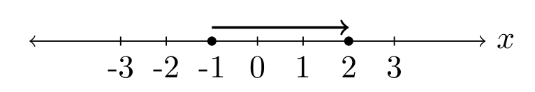
Above we showed that the differential equation $dx = \frac{dx}{du}du$ tells us how to relate lengths along the $u$-axis to lengths along the $x$-axis. We could think of the number $\frac{dx}{du}$ as a length stretch factor. Let's now examine a two dimensional change-of-coordinates, and connect areas in the $uv$-plane to areas in the $xy$-plane.

2. Consider the change-of-coordinates $x=u-v$ and $y=u+v$, which we could also write as the coordinate transformation $\vec T(u,v) = (u-v,u+v)$.
   1. In the table below, you're given several $(u,v)$ points. Find the corresponding $(x,y)$ pair. $$ \begin{array}{|c|c|c|} \text{Name}&(u,v)&(x,y)\\\hline A&(0,0)&(0,0)\\ B&(1,0)&(1-0,1+0) = (1,1)\\ C&(0,1)&(0-1,0+1) = (-1,1)\\ D&(1,1)&\\ E&(3,3)&\\ F&(2,4)&\\ G&(-2,4)&\\ \end{array}$$
   2. There are two graphs below. One is a plot in the $uv$-plane of the points from the table, along with the parabola $v=u^2$, the line $v=u$, and the shaded box whose corners are the first four points. Complete a similar plot in the $xy$-plane by adding the remaining points, and then connect the points in your $xy$ plot to show how the parabola, line, and shaded box (done for you) transform because of this change-of-coordinates. How would you describe what this change-of-coordinates is doing?
      • 
      • The following Mathematica code allows you to draw any region from the $uv$-plane in the $xy$ plane. You can use it to check your work (as well as adapt the code to work with ANY new coordinate system).

        R1 = ParametricRegion[{{u - v, u + v}, 0 <= u <= 1 && 0 <= v <= 1}, {u, v}];
        Region[R1, Axes -> True, AxesLabel -> {x, y}]
        
        R2 = ParametricRegion[{{u - v, u + v}, v == u^2}, {{u, -2, 2}, v}];
        Region[R2, Axes -> True, AxesLabel -> {x, y}]
        

   3. The differential of $x$ is $dx = du-dv$. Obtain a similar formula for the differential $dy$. Then write your answer as the vector equation (linear combination) $$\begin{pmatrix}dx\\dy\end{pmatrix} = \begin{pmatrix} 1\\ ?\end{pmatrix}du+\begin{pmatrix}-1\\?\end{pmatrix}dv.$$
   4. How are areas in the $uv$-plane related to areas in the $xy$-plane? In particular, the area of the 1 by 1 box in the $uv$ plane is 1. What is the area of the shaded region in the $xy$-plane. By how much are we stretching areas when we change from $uv$ to $xy$ coordinates (what's the "area stretch factor")?

The area stretch factor above is called a "Jacobian". We'll soon have quick way to compute a Jacobian, which will result from finding the area of a parallelogram (the next task).

Task 33.2

We need a quick way to compute the area of a parallelogram. In this task, we'll prove the following theorem and then use it in a few specific examples.

1. Suppose a parallelogram has edges that are parallel to the vectors $\vec u=(a,b)$ and $\vec v=(c,d)$. Prove that the area of this parallelogram is given by $|ad-bc|$. If you want some help, here are some steps you can follow:
   1. Draw a generic parallelogram. Label one corner the origin, and then the two connecting edges are the vectors $\vec u = (a,b)$ and $\vec v=(c,d)$.
   2. Add to your picture (1) the projection of $\vec u$ onto $\vec v$ (so $\vec u_{\parallel \vec v}$) and (2) the component of $\vec u$ that is orthogonal to $\vec v$ (so $\vec u_{\perp \vec v}$).
   3. Explain why the area is $A = |\vec v||\vec u_{\perp \vec v}|$.
   4. Use Mathematica to perform the computations, and then explain why the result given is equal to $|ad-bc|$.

      u = {a, b};
      v = {c, d};
      uPerpv = u - Projection[u, v];
      Norm[uPerpv]*Norm[v] // FullSimplify
      
2. Whether you are able to complete the proof above or not, let's practice using the result to compute areas of parallelogram (and triangles). Use the area formula $|ad-bc|$ to compute the requested areas below.
   1. A parallelogram has vertices $(0,0)$, $(-2,5)$, $(3,4)$, and $(1,9)$. Find its area.
   2. Find the area of the triangle with vertices $(0,0)$, $(-2,5)$, and $(3,4)$.
   3. Find the area of the triangle with vertices $(-3,1)$, $(-2,5)$, and $(3,4)$. [You'll need to give vectors $\vec u$ and $\vec v$ that form the edges of a parallelogram.]

Task 33.3

Recall that the gradient of a function $f$ is the quantity $$\vec \nabla f = \left(\frac{\partial f}{\partial x},\frac{\partial f}{\partial y},\frac{\partial f}{\partial z} \right) = \left(\frac{\partial }{\partial x},\frac{\partial }{\partial y},\frac{\partial }{\partial z} \right)f ,$$ where in the last expression we let $\vec \nabla = \left(\frac{\partial }{\partial x},\frac{\partial }{\partial y},\frac{\partial }{\partial z} \right)$ and then treat $\vec \nabla f$ as a "vector" $\vec \nabla$ times a scalar $f$. The quantity $\vec \nabla = \left(\frac{\partial }{\partial x},\frac{\partial }{\partial y},\frac{\partial }{\partial z} \right)$ is an example of something we call an "operator," something that operates on functions.

We've already encountered several operators before this class. For example, the derivative operator $\frac{d}{dx}$ from first semester calculus takes a function such as $f(x) = x^2$ and returns a new function $\frac{d}{dx}f = 2x$. The integral operator $\int_a^b f dx$ takes a function $f$ and return a real number. The gradient operator takes a function $f$ and returns a vector of functions $\vec \nabla f = (f_x,f_y,f_z)$. This is just 3 examples of operators. Here are two more.

Use the definitions above to compute the divergence and curl of each vector field below. Then compute the derivative (which will be a 3 by 3 matrix). Finish by checking your work with Mathematica (code for doing so is provided below). If you see any relationships worth mentioning, articulate them in your work.

1. $\vec F = (2x, 3y^2, e^z)$
2. $\vec F = (-3y, 3x, 5z)$
3. $\vec F = (z-3y, 3x, -x)$

In class, we'll talk about the physical meaning of each result above.

F = {x^2 y, x y z, 3 x + 4 z }
D[F, {{x, y, z}}] // MatrixForm
Div[F, {x, y, z}]
Curl[F, {x, y, z}]

Task 33.4

Pick some problems related to the topics we are discussing from the Text Book Practice page.

Prep.Day34

Task 34.1

It's time to focus on how area is changed when we perform a change-of-coordinates. We'll see that finding the area of a transformed parallelogram is the key.

1. Consider the change-of-coordinates $x=2u$, $y=3v$.
   1. The lines $u=0,u=1,u=2$ and $v=0,v=1,v=2$ correspond to lines in the $xy$-plane. Draw these lines in the $xy$-plane (the line $v=1$ is done for you).
      • 
   2. The box in the $uv$-plane with $0\leq u\leq 1$ and $1\leq v\leq 2$ corresponds to a box in the $xy$-plane. Shade this box in the $xy$-plane and find its area.
   3. Compute the differentials $dx$ and $dy$. State them using the vector form (linear combination) $$\begin{pmatrix}dx\\dy\end{pmatrix} = \begin{pmatrix} ?\\ ?\end{pmatrix}du+\begin{pmatrix}?\\?\end{pmatrix}dv$$ What do the two vectors $(a,0)$ and $(0,b)$ have to do with your picture?
   4. Draw the box given by $-1\leq u\leq 1$ and $-1\leq v\leq 1$ in both the $uv$-plane and $xy$-plane. Then state the area $A_{uv}$ of this box in the $uv$-plane, and state the area $A_{xy}$ of the corresponding rectangle in the $xy$-plane.
   5. Consider the circle $u^2+v^2=1$, whose area inside is $A_{uv}=\pi$. Guess the area $A_{xy}$ inside the corresponding ellipse in the $xy$-plane. Explain.
2. Consider now the change-of-coordinates $x=2u+v$, $y=u-2v$.
   1. The lines $u=0,u=1,u=2$ and $v=0,v=1,v=2$ correspond to lines in the $xy$ plane. Draw these lines in the $xy$-plane (the line $v=1$ is drawn for you). One option is to find the $xy$ coordinates of the $(u,v)$ points $(0,0)$, $(0,1)$, $(0,2)$, $(1,0)$, $(1,1)$, etc., and then just connect the dots to make a rotated grid.
      • 
   2. The box in the $uv$-plane with $0\leq u\leq 1$ and $1\leq v\leq 2$ should correspond to a parallelogram in the $xy$ plane. Shade this parallelogram in your picture above.
   3. Compute the differentials $dx$ and $dy$. State them using the vector form (linear combination) $$\begin{pmatrix}dx\\dy\end{pmatrix} = \begin{pmatrix} ?\\ ?\end{pmatrix}du+\begin{pmatrix}?\\?\end{pmatrix}dv.$$ What do the two vectors above have to do with your picture?
   4. Show that the area of the parallelogram formed using these two vectors is 5. How would you describe the change in area between the graph in the $uv$-plane, and the graph in the $xy$-plane?

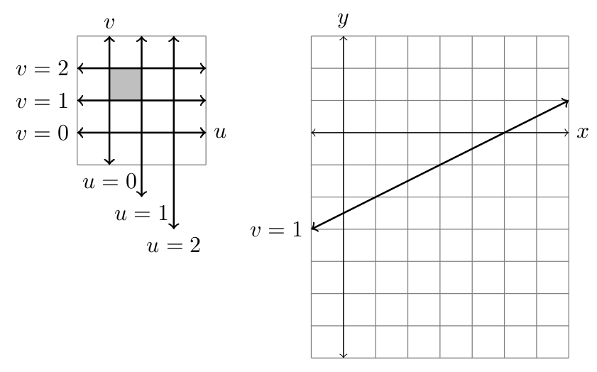
The following code will help you check that your work on the second part is correct.

coordinates = {2 u + v, u - 2 v}
R = ParametricRegion[{coordinates, 0 <= u <= 1 && 1 <= v <= 2}, {u, v}];
Region[R, Axes -> True, AxesLabel -> {x, y}, AxesOrigin -> {0, 0}]
R = ParametricRegion[{coordinates, u == 0 || u == 1 || u == 2 || v == 0 || v == 1 || v == 2}, {{u, -1, 3}, {v, -1, 3}}];
Region[R, Axes -> True, AxesLabel -> {x, y}, AxesOrigin -> {0, 0}]

Task 34.2

Many vector fields are the derivative of a function. This function we call a potential for the vector field. Once we are comfortable finding potentials, we'll show that the work done by a vector field with a potential is the difference in the potential.

Let's practice finding gradients and potentials. You're welcome to watch this YouTube Video before starting, or just jump in and give it a try.

1. Let $f(x,y) = x^2+3xy+2y^2$. Find $\vec \nabla f$. Then compute $D^2f(x,y)$ (you should get a square matrix). What are $f_{xy}$ and $f_{yx}$?
2. Consider the vector field $\vec F(x,y)=(2x+y,x+4y)$. Find the derivative of $\vec F(x,y)$ (it should be a square matrix). Then find a function $f(x,y)$ whose gradient is $\vec F$ (i.e. $Df=\vec F$). What are $f_{xy}$ and $f_{yx}$?
3. Consider the vector field $\vec F(x,y)=(2x+y,3x+4y)$. Find the derivative of $\vec F$. Why is there no function $f(x,y)$ so that $Df(x,y)=\vec F(x,y)$? [Hint: look at $f_{xy}$ and $f_{yx}$.]

4. For each of the following vector fields, start by computing the derivative. Then find a potential, or explain why none exists.
   1. $\vec F(x,y)=(2x-y, 3x+2y)$
   2. $\vec F(x,y)=(2x+4y, 4x+3y)$
   3. $\vec F(x,y)=(2x+4xy, 2x^2+y)$
   4. $\vec F(x,y,z)=(x+2y+3z,2x+3y+4z,2x+3y+4z)$
   5. $\vec F(x,y,z)=(x+2y+3z,2x+3y+4z,3x+4y+5z)$
   6. $\vec F(x,y,z)=(x+yz,xz+z,xy+y)$

The Mathematica code below starts by computing the derivative $D\vec F$, then uses DSolve to find a potential, and finishes by computing the gradient of the potential to see if it is the original vector field (verify you have the correct solution). If a potential exists, then the last line should match the first. You'll need to add a third variable (,z) in appropriate spots to use this code for a 3D vector field.

ClearAll[F, f, x, y]
F = {2 x + y, x + 4 y}
D[F, {{x, y}}] // MatrixForm
potential = DSolve[D[f[x, y], {{x, y}}] == F, f[x, y], {x, y}]
D[f[x, y] /. potential, {{x, y}}] // Flatten

Task 34.3

We already found the area of parallelogram in the $xy$-plane. To use new coordinate systems in 3D, we'll need to volume of a parallelepiped formed by the three vectors $\vec u$, $\vec v$, and $\vec w$, shown in the image below.

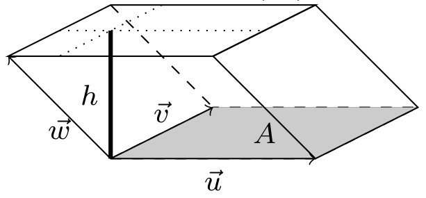
We get the volume by obtaining the area $A$ of one face, multiplied by the distance $h$ between the base and the plane containing the opposing face. This means we need to (1) compute the area of a parallelogram in 3D, and then (2) obtain a formula for the distance between the opposing faces. In this task, we'll see that the cross product and dot product provide us with precisely the tools we need to do both tasks.

1. Let $\vec u = (a,b,c)$ and $\vec v = (d,e,f)$. Our goal is to find the area of a parallelogram whose edges are formed from these two vectors.
   1. Draw a picture that contains 2 vectors labeled $\vec u$ and $\vec v$. In that picture, include $\vec u_{\parallel \vec v}$ and $\vec u_{\perp\vec v}$. Explain why the area we seek is $A = |\vec u_{\perp\vec v}||\vec v|$. Then use the following Mathematica code to compute the area. The Assumptions command below is needed to help Mathematica do some simplifications .

      $Assumptions = a \[Element] Reals && b \[Element] Reals && c \[Element] Reals && d \[Element] Reals && e \[Element] Reals && f \[Element] Reals;
      u = {a, b, c};
      v = {d, e, f};
      uPerpv = u - Projection[u, v];
      Norm[uPerpv]*Norm[v] // Simplify
      

   2. The magnitude of the cross product is $$|\vec u\times \vec v|= |(bf-ce, cd-af, ae-bd)| = \sqrt{(bf-ce)^2+ (cd-af)^2+ (ae-bd)^2}.$$ Show that the magnitude of the cross product and the area of the parallelogram (the value you obtained above) are the same. You can do this by hand, or with Mathematica. If you choose to use Mathematica, here is code for getting the magnitude of the cross product.

      Norm[Cross[u, v]] // Simplify
      

   3. Use what you just learned to find the area of the parallelogram formed by the two vectors $(1,2,3)$ and $(-3,1,4)$.

Now that we have a formula for the area of one face of a parallelepiped, we only need to find the distance between opposing faces to obtain the volume.

2. Consider three vectors $\vec u$, $\vec v$, and $\vec w$ in $\mathbb{R}^3$. We will find the volume of the parallelepiped formed by these three vectors. Let the base of the parallelogram be the face formed by $\vec u$ and $\vec v$. The height $h$ is the distance between the plane that contains the base and the plane that contain the opposing side of the parallelepiped.
   1. Give a formula to compute the area of the base of the parallelogram. (What did the first part of this tasks help us learn)
   2. Give a vector $\vec n$ that is normal to the base.
   3. Use the projection formula, with the vectors $\vec w$ and $\vec n$ in an appropriate manner, to state the height $h$ of the parallelogram in terms of dot products.
   4. Use your work above to explain why the parallelepiped's volume is $$V=|(\vec u\times \vec v)\cdot \vec w|.$$

Task 34.4

Pick some problems related to the topics we are discussing from the Text Book Practice page.

Prep.Day35

Task 35.1

1. Use the area of a parallelogram formula we developed to explain why the Jacobian can be computed using the formula $$\frac{\partial (x,y)}{\partial (u,v)} = \left|\frac{\partial x}{\partial u}\frac{\partial y}{\partial v}-\frac{\partial x}{\partial v}\frac{\partial y}{\partial u}\right|.$$
2. For the polar coordinate transformation given by the change-of-coordinates $x=r\cos\theta$ and $y=r\sin\theta$, compute the differential $(dx,dy)$, and then show that the Jacobian is $\ds\frac{\partial (x,y)}{\partial (r,\theta)} = |r|$. This is precisely the reason we use the notation $dA = |r|drd\theta$ when setting up double integrals using polar coordinates.
3. For the change-of-coordinates $x=2u-v$ and $y=u+2v$, compute the differential $(dx,dy)$, and then obtain the Jacobian $\ds \frac{\partial (x,y)}{\partial (u,v)}$.
4. For the change-of-coordinates $x=au$ and $y=bv$, show that the Jacobian is $\ds \frac{\partial (x,y)}{\partial (u,v)}=|ab|$.
5. For the change-of-coordinates $u=x+y$ and $v=x-y$, show that $\ds \frac{\partial (u,v)}{\partial (x,y)} = 2$.
6. For the change-of-coordinates $u=x+y$ and $v=x-y$, first solve for $x$ and $y$ in terms of $u$ and $v$ (so obtain $x = ....$ and $y= ...$). Then show that $\ds \frac{\partial (x,y)}{\partial (u,v)} = \frac{1}{2}$.

Did you notice that $\ds \frac{\partial (u,v)}{\partial (x,y)} = \left(\ds \frac{\partial (x,y)}{\partial (u,v)}\right)^{-1}$?

Task 35.2

In three dimensions, some common coordinate systems are cylindrical and spherical coordinates. In this task, for each of these coordinates systems, we'll (1) develop the change-of-coordinates formula, (2) compute the Jacobian using the triple product, and then (3) use the Jacobian to compute the volume of an object in this coordinate system.

Let's first tackle cylindrical coordinates. Let $P=(x,y,z)$ be a point in space. This point lies on a cylinder of radius $r$, where the cylinder has the $z$ axis as its axis of symmetry. The height of the point is $z$ units up from the $xy$ plane. The point casts a shadow in the $xy$ plane at $Q=(x,y,0)$. The angle between the ray $\vec{Q}$ and the $x$-axis is $\theta$. See the image below.

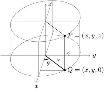
1. Explain why the equations for cylindrical coordinates are $$x=r\cos\theta, \quad y=r\sin\theta,\quad z=z.$$ [Hint: Compute the sine and cosine of $\theta$ in terms of $x$, $y$, and $r$, and then solve for $x$ and $y$.]
2. Compute the Jacobian $\dfrac{\partial(x,y,z)}{\partial(r,\theta,z)}$ for cylindrical coordinates. The steps below are a guide, if needed.
   • For cylindrical coordinates we have $x=r\cos\theta$, $y=r\sin\theta$, and $z=z$. Write the differential $d(x,y,z)$ as the linear combination of partial derivatives $$\begin{pmatrix}dx\\dy\\dz\end{pmatrix} = \begin{pmatrix}\cos\theta\\\sin\theta\\0\end{pmatrix}dr+\begin{pmatrix}?\\?\\?\end{pmatrix}d\theta+\begin{pmatrix}?\\?\\?\end{pmatrix}dz.$$
   • Compute the volume of the parallelepiped formed by the three vectors (partial derivatives) above, using the triple product. Software can make quick work of this. Simplify your result to show that $\dfrac{\partial(x,y,z)}{\partial(r,\theta,z)} = |r|$.
3. Consider the solid domain $D$ in space that lies inside the right circular cylinder $x^2+y^2=a^2$ (or $r=a$) for $0\leq z\leq h$. Start by drawing the domain $D$. The volume in cylindrical coordinates is given by the iterated integral $$V = \iiint_D dV = \ds\int_{0}^{2\pi}\int_{0}^{a}\int_{0}^{h}rdzdrd\theta.$$ Compute this integral to obtain a familiar formula $V = \pi a^2 h$.

Now let's tackle spherical coordinates. Let $P=(x,y,z)$ be a point in space. This point lies on a sphere of radius $\rho$ ("rho"), where the sphere's center is at the origin $O=(0,0,0)$. The point casts a shadow in the $xy$ plane at $Q=(x,y,0)$. The angle between the ray $\vec{Q}$ and the $x$-axis is $\theta$, which some call the azimuth angle. The angle between the ray $\vec{P}$ and the $z$-axis is $\phi$ ("phi"), which some call the inclination angle, polar angle, or zenith angle. See the image below.

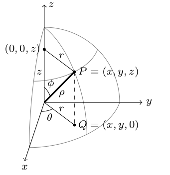
4. Explain why the equations for spherical coordinates are $$x=\rho\sin\phi\cos\theta,\quad y=\rho\sin\phi\sin\theta,\quad z=\rho\cos\phi.$$ [Hint: Compute the sine and cosine of $\phi$ in terms of $\rho$, $r$, and $z$, and then solve for $r$ and $z$. Substitution into $x=r\cos\theta$ and $y=r\sin \theta$ will get the rest.]
5. Compute the Jacobian $\dfrac{\partial(x,y,z)}{\partial(\rho,\phi,\theta)}$ for spherical coordinates. The steps below are a guide, if needed.
   • For spherical coordinates we have $$x=\rho\sin\phi\cos\theta,\quad y=\rho\sin\phi\sin\theta,\quad z=\rho\cos\phi.$$ Write $d(x,y,z)$ as a linear combination of partial derivatives, so $$\begin{pmatrix}dx\\dy\\dz\end{pmatrix} = \begin{pmatrix}\sin\phi\cos\theta\\\sin\phi\sin\theta\\\cos\phi\end{pmatrix}d\rho+\begin{pmatrix}?\\?\\?\end{pmatrix}d\phi+\begin{pmatrix}?\\?\\?\end{pmatrix}d\theta.$$
   • Compute the volume of the parallelepiped formed by the three vectors (partial derivatives) above. Software can make quick work of this. You can do it all by hand, but you'll have to use a Pythagorean identity several times to complete the simplification. Simplify your result to show that $\frac{\partial(x,y,z)}{\partial(\rho,\phi,\theta)} = |\rho^2\sin\phi|$.
6. Consider the solid domain $D$ in space that lies inside the sphere $x^2+y^2+z^2=a^2$ (or $\rho=a$). Start by drawing the domain $D$. The volume in spherical coordinates is given by the iterated integral $$V = \iiint_D dV = \ds\int_{0}^{2\pi}\int_{0}^{\pi}\int_{0}^{a}\rho^2\sin\phi d\rho d\phi d\theta.$$ Compute this integral to obtain a familiar formula $V = \frac{4}{3}\pi a^3$.

Task 35.3

For a differentiable function $f(x)$, the second part of the fundamental theorem of calculus states that $\ds\int_a^b \frac{df}{dx} dx =f(b)-f(a)$. To find the total change in a function $f$ (so $f(b)-f(a)$), we just sum the little changes $\int_C df = \int_C \frac{df}{dx}dx$. We'll use this fact to greatly simplify work computations for vector fields that have a potential.

Let $\vec F$ be a vector field with $f$ being a potential for $\vec F$, meaning $\vec F = \vec \nabla f$. Let $\vec r(t)$ for $a\leq t\leq b$ be a differentiable parametrization of a curve $C$. Let $A = \vec r(a)$ and $B= \vec r (b)$ be the end points of the curve. The composite function $g(t) = f(\vec r(t)) = (f\circ \vec r)(t)$ gives the potential at points along the curve. In particular $f(A)$ and $f(B)$ give the potential at the end points of the curve. The difference in potential is $f(B)-f(A)$.

1. Pause. Reread the above. Do you understand what each of $\vec F$, $f$, $\vec r$, $a$, $b$, $A$, $B$, and $g$ represent? If not, what parts do you have questions about? Then continue reading.

From the chain rule, the composite function $g(t) = f(\vec r(t)) = (f\circ \vec r)(t)$ has the derivative $\frac{dg}{dt}=\vec \nabla f(\vec r(t))\cdot\frac{d\vec r}{dt}$. We now compute $$\begin{align*} f(B)-f(A) &= f(\vec r(b))-f(\vec r(a))&\text{($A$ and $B$ are the end points of the curve)}\\ &= g(b)-g(a)&\text{(recall $g(t) = f(\vec r(t))$}\\ &= \int_a^b \frac{dg}{dt}dt&\text{(the fundamental theorem of calculus)}\\ &= \int_a^b \vec \nabla f(\vec r(t))\cdot \frac{d\vec r}{dt} dt&\text{(using the chain rule to compute $\frac{dg}{dt}$)}\\ &= \int_C \vec F\cdot d\vec r&\text{(recall that $\vec \nabla f=\vec F$)}. \end{align*}$$ This shows that the work done by $\vec F$ along $C$ is the difference in the potential $f$.

Let's try using this theorem in a few situations.

2. Let $\vec F(x,y) = (2x+y,x+4y)$ and $C$ be the parabolic path $\vec r(t) = (t,9-t^2)$ for $-3\leq t\leq 2$.
   1. Use the work formula we developed earlier in the semester, so $\int_C Mdx+Ndy$ or $\int_C \vec F\cdot d\vec r$, to set up and compute the work done by $\vec F$ along $\vec r$. This is a review of a previous learning target. Feel free to use software to complete the integral.
   2. Find a potential $f$ for $\vec F$, state $A$ and $B$, and then compute $f(B)-f(A)$.
   3. Identify the function $g(t) = f(\vec r(t))$, compute $\frac{dg}{dt}$, state $\vec F(\vec r(t))$ and $\frac{d\vec r}{dt}$, and then verify that $\frac{dg}{dt} = \vec F(\vec r(t))\cdot \frac{d\vec r}{dt}$ (these were the terms that appeared in the proof of the fundamental theorem of line integrals).
3. Let $\vec F(x,y,z) = (2x+yz,2z+xz,2y+xy)$ and $C$ be the straight segment from $(2,-5,0)$ to $(1,2,3)$. Compute the work done by $\vec F$ along $C$ by first finding a potential for $\vec F$.
4. Let $\vec F = (x,2yz,y^2)$. Let $C$ be the curve which starts at $(1,0,0)$ and follows a helical path $(\cos t, \sin t, t)$ to $(1,0,2\pi)$ and then follows a straight line path to $(2,4,3)$. Find the work done by $\vec F$ to get from $(1,0,0)$ to $(2,4,3)$ along this path.
5. Suppose a vector field $\vec F$ has a potential. Compute $\int_C \vec F\cdot d\vec r$ where $C$ is the path parametrized by $\vec r(t) = (3\cos t, 3\sin t)$ for $0\leq t\leq 2\pi$.

Task 35.4

Pick some problems related to the topics we are discussing from the Text Book Practice page.

Prep.Day36

Task 36.1

This task has you practice using spherical and cylindrical coordinates. Mathematica's ParametricRegion[] command allows us to plot a region, using any coordinate system, which is extremely useful for visualizing regions defined by bounds of an integral. As an example, the code below visualizes the region whose volume is given by the cylindrical coordinate iterated triple integral $$\int_{1}^{3}\int_{\pi/2}^{2\pi}\int_{0}^{r}rdz d\theta dr,$$ and then computes the triple integral.

coordinates = {r Cos[theta], r Sin[theta], z}
R = ParametricRegion[coordinates, {{r, 1, 3}, {theta, Pi/2, 2 Pi}, {z, 0, r}}];
Region[R, Axes -> True, AxesLabel -> {x, y, z}, AxesOrigin -> {0, 0, 0}]
Integrate[r, {r, 1, 3}, {theta, Pi/2, 2 Pi}, {z, 0, r}]

To compute integrals in spherical coordinates, we just update the change-of-coordinates and bounds. Here's code to plot the region whose volume is given by the spherical coordinate iterated triple integral $$\ds \int_{0}^{\pi}\int_{\pi/6}^{\pi/3}\int_{1}^{3}\rho^2\sin\phi d\rho d\phi d\theta.$$

coordinates = {rho Sin[phi] Cos[theta], rho Sin[phi] Sin[theta], rho Cos[phi]}
R = ParametricRegion[coordinates, {{theta, 0, Pi/2}, {phi, Pi/6, Pi/3}, {rho, 1, 3}}];
Region[R, Axes -> True, AxesLabel -> {x, y, z}, AxesOrigin -> {0, 0, 0}]
Integrate[rho^2 Sin[phi], {theta, 0, Pi/2}, {phi, Pi/6, Pi/3}, {rho, 1, 3}]

1. Consider the solid domain $D$ in space which is above the cone $z=\sqrt{x^2+y^2}$ and below the paraboloid $z=6-x^2-y^2$.
   1. Sketch the region by hand.
   2. Explain why an equation of the cone in cylindrical coordinates is $z=r$. Then obtain an equation of the paraboloid in cylindrical coordinates.
   3. Use cylindrical coordinates to set up an iterated triple integral that would give the volume of the region. You'll need to find where the surfaces intersect, as their intersection will help you determine the appropriate bounds. Use the ParametricRegion[] command to verify that the bounds you gave do indeed produce the correct region.
   4. By symmetry, it should be clear that for the centroid of this region, we have $\bar x = \bar y = 0$. Set up a formula involving iterated triple integrals that would give $\bar z$ for this solid, and then use software to compute $\bar z$.
2. Consider the solid domain $D$ in space that lies below the cone $z=\sqrt{x^2+y^2}$, above the $xy$-plane, and inside the sphere $x^2+y^2+z^2=25$.
   1. Provide a sketch of the domain $D$.
   2. Explain why an equation of the cone in spherical coordinates is $\phi = \pi/4$. Then given an equation of the sphere in spherical coordinates.
   3. Set up an integral in spherical coordinates that gives the volume of $D$. Use the ParametricRegion[] command to verify that the bounds you gave do indeed produce the correct region.
   4. Set up an integral in spherical coordinates that would give the $z$-coordinate of the centroid of $D$.

Task 36.2

Two important vector fields show up over and over again when studying gravity and electrostatics. In this task we will develop a common formula for these fields, show that these fields have a potential, and then practice using the fundamental theorem of line integrals to perform work computations, using the potential.

1. We need a formula for a vector field where at each point in space, the vector points towards the origin with a magnitude that proportional to 1 over the square of the distance to the origin. To obtain this field, complete the following steps.
   1. Let $P=(x,y,z)$ be a point in space. At the point $P$, let $\vec F_1(x,y,z)$ be the vector which points from $P$ to the origin. Give a formula for $\vec F_1(x,y,z)$.
   2. Give an equation of the vector field where at each point $P$ in space, the vector $\vec F_2(P)$ is a unit vector that points towards the origin.
   3. Give an equation of the vector field where at each point $P$ in space, the vector $\vec F_3(P)$ is a vector of length 7 that points towards the origin.
   4. Give an equation of the vector field where at each point $P$ in space, the vector $\vec F(P)$ points towards the origin, and has a magnitude equal to $G/d^2$ where $d = \sqrt{x^2+y^2+z^2}$ is the distance to the origin, and $G$ is a constant.
2. The gravitational vector field is directly related to the radial field $\ds\vec F(x,y,z) = \frac{\left(-x,-y,-z\right)}{(x^2+y^2+z^2)^{3/2}}$.
   1. We say that a vector field is conservative when the work done by the field is independent of the path traveled. Show that this vector field is conservative, by finding a potential for $\vec F$.
   2. Compute the work done by $\vec F$ to move an object from $(1,2,-2)$ to $(0,-3,4)$ along ANY path that avoids the origin.

Task 36.3

We need to gain some familiarity with the notation related to gradients, divergence, and curl. As you work on the tasks below, you are welcome to use subscript notation (such as $f_x$ and $M_y$) to simplify writing.

1. Suppose $f(x,y,z)$ is twice continuously differentiable.
   1. Compute the curl of the gradient of $f$, so compute $\vec \nabla \times \vec \nabla f$. Simplify the result as much as possible.
   2. If a vector field $\vec F = (M,N,P)$ has a potential, then what is the curl of $\vec F$?
2. Suppose $\vec F(x,y,z) = (M,N,P)$ is a vector field and $f(x,y,z)$ is a function, both of which are twice continuously differentiable.
   1. Compute the divergence of the curl of $\vec F$, so compute $\vec \nabla \cdot \left(\vec \nabla \times \vec F\right)$, and simplify the result as much as possible.
   2. Compute the divergence of the gradient of $f$, so compute $\vec \nabla \cdot \vec \nabla f$, and simplify the result as much as possible.

Task 36.4

Pick some problems related to the topics we are discussing from the Text Book Practice page.

Prep.Day37

Task 37.1

1. Consider the region that lies below the $z$-axis and between 2 spheres of radii $a$ and $b$ with $a<b$. The image below shows such a region where the inner radius is $a=3$, and the outer radius is $b=5$.
   • 
   1. Set up an iterated triple integral in spherical coordinates to compute the volume of this region.
   2. Set up an iterated triple integral formula to compute the $z$-coordinate of the centroid (symmetry gives us $\bar x = \bar y = 0$).
   3. If the temperature at points in this region is given by $T(x,y,z) = x+3$, then set up an iterated triple integral formula that would give the average temperature of the region.
2. A metal casing lies inside the cylinder $x^2+y^2=4$, outside the cylinder $x^2+y^2=1$, below the paraboloid $z=9-x^2-y^2$, and above the plane $z=0$. The region is shown below, where one quarter of the region was removed so you can see the hollow interior.
   • 
   1. Set up an iterated integral in cylindrical coordinates to compute the volume of the casing.
   2. The casing is made of a composite material and the density of the casing is more dense the further from the center. The density is given by $\delta(x,y,z) = x^2+y^2$. Set up an iterated triple integral formula to compute the $z$-coordintate of the center-of-mass of the casing.

Remember that you can verify that your bound are correct by using Mathematica to draw whatever you decide the bounds should be. Here's two examples of how to construct regions, the first in cylindrincal coordinates, and the second in spherical coordinates.

coordinates = {r Cos[theta], r Sin[theta], z}
R = ParametricRegion[coordinates, {{r, 1, 3}, {theta, Pi/2, 2 Pi}, {z, 0, r}}];
Region[R, Axes -> True, AxesLabel -> {x, y, z}, AxesOrigin -> {0, 0, 0}]
Integrate[r, {r, 1, 3}, {theta, Pi/2, 2 Pi}, {z, 0, r}]

coordinates = {rho Sin[phi] Cos[theta], rho Sin[phi] Sin[theta], rho Cos[phi]}
R = ParametricRegion[coordinates, {{theta, 0, Pi/2}, {phi, Pi/6, Pi/3}, {rho, 1, 3}}];
Region[R, Axes -> True, AxesLabel -> {x, y, z}, AxesOrigin -> {0, 0, 0}]
Integrate[rho^2 Sin[phi], {theta, 0, Pi/2}, {phi, Pi/6, Pi/3}, {rho, 1, 3}]

If the code above is extremely slow on your computer, then you can use the code below instead. The code is more complicated, as it plots the six surfaces defined by the bounds you choose, but the code used requires very minimal processing (it works fast). (The Evaluate[] command is needed for the code to work prior to Mathematica 13.)

plotRegion3D[cs_, ob_, mb_, ib_] := 
 Show[{{ParametricPlot3D[Evaluate[Table[cs /. (ib[[1]] -> ib[[i]]), {i, 2, 3}], ob, mb], AxesLabel -> {x, y, z}, Mesh -> {15, 1}], 
    ParametricPlot3D[Evaluate[Table[(cs /. (ib[[1]] -> (ib[[2]] (1 - s) + ib[[3]] s))) /. (mb[[1]] -> mb[[i]]), {i, 2, 3}], ob], {s, 0, 1}, PlotStyle -> {Red, Blue}, Mesh -> {15, 0}], 
    ParametricPlot3D[Evaluate[Table[(cs /. (ib[[1]] -> (ib[[2]] (1 - s) + ib[[3]] s))) /. (mb[[1]] -> (mb[[2]] (1 - t) + mb[[3]] t)) /. (ob[[1]] -> ob[[i]]), {i, 2, 3}]], {t, 0, 1}, {s, 0, 1}, PlotStyle -> Green, Mesh -> {0, 0}]}}, PlotRange -> All]

coordinates = {r Cos[theta], r Sin[theta], z}
plotRegion3D[coordinates, {r, 1, 3}, {theta, Pi/2, 2 Pi}, {z, 0, r}]

coordinates = {rho Sin[phi] Cos[theta], rho Sin[phi] Sin[theta], rho Cos[phi]}
plotRegion3D[coordinates, {theta, 0, Pi/2}, {phi, Pi/6, Pi/3}, {rho, 1, 3}]

Much simpler code will draw 2D regions

plotRegion[cs_, ob_, ib_] := ParametricPlot[Evaluate[cs, ob, ib], Mesh -> {10, 0}]

coordinates = {r Cos[theta], r Sin[theta]};
plotRegion[coordinates, {theta, Pi/4, Pi}, {r, 2, 5}]

Task 37.2

1. Consider the region $R$ in space satisfying $0\leq x-y\leq 4$ and $1\leq 2x+y\leq 3$. We wish to evaluate the integral $\ds\iint_R xy dA$.
   1. Draw the region $R$.
   2. Using the change-of-coordinates $u=x-y$ and $v=2x+y$, compute the Jacobian $\frac{\partial(u,v)}{\partial (x,y)}$.
   3. Find $x$ and $y$ in terms of $u$ and $v$.
   4. Use this change-of-coordinates to compute $\ds\iint_R xy dA$ by first setting up an appropriate iterated integral of the form $\ds \int_{?}^{?}\int_{?}^{?}?dudv$.
2. Consider the ellipsoid $\ds\frac{x^2}{a^2}+\frac{y^2}{b^2}+\frac{z^2}{c^2}=1$, for some positive constants $a$, $b$, and $c$.
   1. Draw the region.
   2. Using the change-of-coordinates $x = a u \sin v \cos w$, $y = b u \sin v \sin w$, $x = c u \cos v$, compute the Jacobian $\frac{\partial (x,y,z)}{\partial (u,v,w)}$. Feel free to use software to help you.
   3. Set up an iterated integral using $uvw$-coordinates to compute the volume inside the ellipsoid. Then compute the integral.
   4. Set up an iterated integral using $uvw$-coordinates to show that $\bar z = \frac{3c}{16}$ for the region inside the ellipsoid that is above the $xy$-plane.

Task 37.3

When you can use a potential to compute work, it greatly simplifies things.

1. As you complete each problem below, first ask if there is a potential.
   1. Compute the work done by the vector field $\vec F(x,y) = (y,x)$ on a object that moves along the path $\vec r(t) = (\cos t, \sin t)$ for $0\leq t\leq 2 \pi$.
   2. Compute the work done by the vector field $\vec F(x,y) = (-y,x)$ on a object that moves along the path $\vec r(t) = (\cos t, \sin t)$ for $0\leq t\leq 2 \pi$.
   3. For each vector field above, use Mathematica to construct an image that shows the vector field along with the curve in the same plot. (You'll need VectorPlot[] and ParametricPlot[], with Show[] to get them in the same plot).

We've seen that if a vector field has a potential, then the derivative is symmetric. Is the converse of this statement true, namely if the derivative of a vector field is symmetric, then does that mean the vector field has a potential?

2. Consider the vector field $\ds\vec F(x,y) = \left(\frac{-y}{x^2+y^2},\frac{x}{x^2+y^2}\right)$.
   1. Show that the derivative is symmetric.
   2. Compute the work done by the vector field $\vec F(x,y)$ on a object that moves along the path $\vec r(t) = (\cos t, \sin t)$ for $0\leq t\leq 2 \pi$.
   3. Explain why $\vec F(x,y)$ does not have a potential.
   4. Look up "simply connected region" (see section 6.3), and explain why the domain of $\ds\vec F(x,y) = \left(\frac{-y}{x^2+y^2},\frac{x}{x^2+y^2}\right)$ is NOT simply connected.

When the domain of a continuously differentiable vector field is simply connected, then the vector field has a potential if and only if the derivative is symmetric. The concept of a simply connected domain is the start of an entire branch of mathematics called algebraic topology, all stemming from the question, "under what circumstances can we guarantee that a vector field will have a potential?"

Task 37.4

Pick some problems related to the topics we are discussing from the Text Book Practice page.

Prep.Day38

Task 38.1

The shell method and disc method are two methods for computing the volume of a solid of revolution using a single integral. As a solid of revolution has volume, then a triple integral will give the volume, provided we can set up appropriate bounds. In this task, we'll see that the only difference between the shell and disc methods are the order in which a triple integral is done. If you've forgotten (which is completely normal), here's a reminder.

• The shell-method computes volumes with $$V = \int dV = \int_a^b \underbrace{(2\pi r)(\text{height of shell at $r$})}_{\text{shell surface area = (circumference)(height)}} \underbrace{dr}_{\text{shell thickness}}.$$
• The disc-method computes volumes with $$V = \int dV =\int_a^b \underbrace{\pi (\text{radius of disc at height $z$})^2}_{\text{area of disc at height $z$}} \underbrace{dz}_{\text{little height}}.$$

1. Consider the solid region in space that is bounded above by $z=9-x^2-y^2$ (so $z=9-r^2$) and below by the $xy$-plane. In Cartesian coordinates, the volume of this region is given by $$\int_{-3}^{3}\int_{-\sqrt{9-x^2}}^{\sqrt{9-x^2}}\int_{0}^{9-x^2-y^2}dzdydx.$$ This region is formed by taking the region under the parabola $z=9-r^2$ (above the plane $z=0$) and revolving it about the $z$-axis.
   1. Set up a triple integral in cylindrical coordinates to compute the volume of this solid using the order $d\theta dzdr$.
   2. Compute the two inside integrals and simplify to show that $V = \int_{0}^{3} 2\pi r (9-r^2) dr$.
   3. Set up a triple integral in cylindrical coordinates to compute the volume of this solid using the order $d\theta drdz$. You will end up with $r=\sqrt{9-z}$ as one of the bounds.
   4. Compute the two inside integrals and simplify to show that $V = \int_{0}^{9} \pi (\sqrt{9-z})^2 dz$.
   5. Which order above uses the shell method, and which uses the disc method?
2. Consider the region in space that satisfies $0\leq a\leq r\leq b$ with $g(r)\leq z\leq f(r)$.
   1. Construct a sketch of such a region. You get to pick and illustrate what $a$, $b$, $g(r)$, and $f(r)$ mean.
   2. Set up a triple integral in cylindrical coordinates to compute the volume of this solid using the order $d\theta dzdr$.
   3. Compute the two inside integrals to obtain a formula for the volume that involves a single integral in terms of $r$.
3. Consider the region in space that satisfies $c\leq z\leq d$ with $0\leq g(z)\leq r\leq f(z)$.
   1. Construct a sketch of such a region. You get to pick and illustrate what $c$, $d$, $g(z)$, and $f(z)$ mean.
   2. Set up a triple integral in cylindrical coordinates to compute the volume of this solid using the order $d\theta drdz$.
   3. Compute the two inside integrals to obtain a formula for the volume that involves a single integral in terms of $z$.

Task 38.2

1. Consider the integral $\ds \int_{0}^{4}\int_{0}^{4-x} e^{(x+y)^2}dydx$ and the change-of-coordinates $u=x$, $v=x+y$.
   1. Solve for $x$ and $y$ in terms of $u$ and $v$, and then compute $\frac{\partial(x,y)}{\partial(u,v)}$.
   2. Set up the corresponding iterated integral using the order $dvdu$. Then set up the corresponding integral using the order $dudv$.
   3. Compute the simpler of the two integrals you just set up.
2. Consider the integral $\ds \iint_R xy dA$ for the region $R$ that lies inside the triangle with vertices $(0,0)$, $(2,4)$, and $(3,-3)$. Notice that two of the edges of the triangle lie on the lines $y=2x$ and $y=-x$, which means we'll use the change-of-coordinates $u=2x-y$, $v=x+y$.
   1. Sketch the region $R$ in the $xy$-plane. Then sketch the corresponding region in the $uv$-plane (you should obtain a triangle).
   2. Set up an iterated integral using $uv$-coordinates to compute $\ds \iint_R xy dA$.
   3. Compute the integral.

Task 38.3

This task focuses on exploring the curl and divergence of a vector field, using Mathematica, to gain some geometric intuition about what these vectors compute.

1. For each vector field below, compute the curl of the vector field, modify this chunk of Mathematica code to visualize the vector field and the curl, and look for relationships between $\vec F$ and $\vec\nabla \times \vec F$.

   F[x_, y_, z_] := {-y, x, 0}
   Show[VectorPlot3D[Evaluate[F[x, y, z]], {x, -1, 1}, {y, -1, 1}, {z, -1, 1}, VectorAspectRatio -> 1/8],
    VectorPlot3D[Evaluate[Curl[F[x, y, z], {x, y, z}]], {x, -1, 1}, {y, -1, 1}, {z, -1, 1}, VectorPoints -> Coarse, VectorAspectRatio -> 1/4]]
   

   1. $\vec F(x,y,z) = (-y,x,0)$
   2. $\vec F(x,y,z) = (-y,x,0)$
   3. $\vec F(x,y,z) = (-z, 0, 2 x)$
   4. $\vec F(x,y,z) = (2x, 3y, 4z)$
   5. $\vec F(x,y,z) = (0, 3 z, -4 y)$
   6. $\vec F(x,y,z) = (-z, z, x - y)$
   7. $\vec F(x,y,z) = (y - z, -x + z, x - y)$
   8. $\vec F(x,y,z) = (y^2, -x, 0)$
   9. Pick your own vector field.
2. Summarize what relationships, if any, you saw.
3. For each vector field below, compute the divergence of the vector field, modify this chunk of Mathematica code to visualize the vector field, and look for relationships between $\vec F$ and $\vec\nabla \cdot \vec F$.

   F[x_, y_, z_] := {2 x, 0, 0}
   VectorPlot3D[Evaluate[F[x, y, z]], {x, -1, 1}, {y, -1, 1}, {z, -1, 1}]
   

   1. $\vec F(x,y,z) = (2x,0,0)$
   2. $\vec F(x,y,z) = (0,-3y,0)$
   3. $\vec F(x,y,z) = (0,0,4z)$
   4. $\vec F(x,y,z) = (2x,-3y,4z)$
   5. $\vec F(x,y,z) = (x,y,z)$
   6. $\vec F(x,y,z) = (-y,x,0)$
   7. $\vec F(x,y,z) = (x^2,0,0)$
   8. Pick your own vector field.
4. Summarize what relationships, if any, you saw.

Task 38.4

Pick some problems related to the topics we are discussing from the Text Book Practice page.

Prep.Day39

There are no new tasks for this day. Work on the tasks from previous days that we have not yet discussed in class.

Prep.Day40

Learning Target Checkoff

A learning target quiz will appear in I-Learn. Complete and submit the quiz before the due date.

Prep.Day41

Task 41.1

We've already learned how to draw parametric space curves, such as $\vec r(t)=(2\cos t, 2\sin t, t)$ for $0\leq t\leq 4\pi$. We pick several values of $t$, plot the corresponding points in space, and then connect the dots. We can draw this function in Mathematica using the following code.

ParametricPlot3D[{2 Cos[t], 2 Sin[t], t}, {t, 0, 4 Pi}]

The example above draws a wire, or path, in space. It's an example of a parametrization that uses only one parameter. Because only one parameter is used, the graph represents an object for which it makes sense to compute lengths. It's like we've wrapped a straight line up in space, using the parametrization. What happens if we increase the number of parameters. That's what this task explores.

1. Suppose a jet begins spiraling upwards to gain height. The position of the jet after $t$ seconds is modeled by the equation $\vec r(t)=(2\cos t, 2\sin t, t).$ The jet is accompanied by several jets flying side by side. As all the jets fly, they leave a smoke trail behind them (it's an air show). The smoke from each jet spreads outwards to mix together, so that it looks like the jets are leaving a wide sheet of smoke behind them as they spiral upwards. The position of two of the many other jets is given by $\vec r_3(t)=(3\cos t, 3\sin t, t)$ and $\vec r_4(t)=(4\cos t,4\sin t,t)$. A function which represents the smoke stream from these jets is $\vec r(a,t)=(a\cos t, a\sin t, t)$ for $0\leq t\leq 4\pi$ and $2\leq a\leq 4$.
   1. Graph the position of the three jets $\vec r(2,t)=(2\cos t, 2\sin t, t)$, $\vec r(3,t)=(3\cos t, 3\sin t, t)$, and $\vec r(4,t)=(4\cos t,4\sin t,t)$ in the same 3D plot.
   2. Let $t=0$ and graph the curve $r(a,0)=(a,0,0)$ for $a\in[2,4]$ (so $2\leq a\leq 4$), which represents a segment along which the smoke has spread. Then repeat this for $t=\pi/2$, then $t=\pi$, and then $t=3\pi/2$.
   3. Describe the resulting surface. Then use Mathematica to view the surface (all it requires is adding another parameter to the code).

      ParametricPlot3D[{a Cos[t], a Sin[t], t}, {t, 0, 4 Pi}, {a, 2, 4}]
      

We call the surface you drew above a parametric surface. The vector equation describing the smoke screen is a parametrization of this surface.

We draw parametric surfaces by joining together many parametric space curves. Pick one variable, hold it constant, and draw the resulting space curve. Repeat this several times, and you'll have a 3D surface plot. Most of 3D computer animation is done using parametric surfaces. Car companies create computer models of vehicles using parametric surfaces, and then use those parametric surfaces to study collisions. Often the mathematics behind these models is hidden in the software program, but parametric surfaces are at the heart of just about every 3D model.

2. Consider the parametric surface $\vec r(u,v)=(u\cos v, u\sin v, u^2)$ for $0\leq u\leq 3$ and $0\leq v\leq 2 \pi$. Construct a graph of this function.
   • Remember, to do so we just let $u$ equal a constant (such as 1, 2, 3) and then graph the resulting space curve where we let $v$ vary. After doing this for several values of $u$, swap and let $v$ equal a constant (such as 0, $\pi/2$, etc.) and graph the resulting space curve as $u$ varies.
   • Did you get a satellite dish? Modify the Mathematica code above to have software construct the surface.

Task 41.2

When a vector has no potential, there is a generalization of the fundamental theorem of calculus that can simplify work computations. To discuss this version (called Green's theorem), we first need a few definitions.

In the definition above, we could have replaced the circle $C_a$ with a square of side lengths $a$ centered at $(x,y)$ with interior area $A_a$. Alternately, we could have chosen any collection of curves $C_a$ which "shrink nicely" to $(x,y)$ and have area $A_a$ inside. Regardless of which curves you chose, it can be shown that $$N_x-M_y=\lim_{a\to 0} \frac{1}{A_a}\oint_{C_a} Mdx+Ndy.$$

To understand what the circulation density mean in a physical sense, think of $\vec F$ as the velocity field of some fluid (a liquid or gas). The circulation density tells us the rate at which the vector field $\vec F$ causes objects to rotate around points. If circulation density is positive, then particles near $(x,y)$ would tend to circulate around the point in a counterclockwise direction. The larger the circulation density, the faster the rotation. The velocity field of a fluid could have some regions where the fluid is swirling clockwise, and some regions where the fluid is swirling counterclockwise.

We are now ready to state Green's Theorem. Ask me in class to give an informal proof as to why this theorem is valid.

Let's use this theorem to find circulation (work on a closed curve).

1. Consider the vector field $\vec F=(2x+3y,4x+5y)$.
   1. Start by computing $N_x-M_y$.
   2. If $C$ is the boundary of the rectangle $2\leq x\leq 7$ and $0\leq y\leq 3$, find the circulation of $\vec F$ along $C$. [Doing this without Green's theorem requires we parametrize 4 line segments, compute 4 integrals, and then sum the results. Green's theorem can make this really fast. ]
   3. Let $R$ be the region inside a circle of radius 3 that is centered at the origin. Compute the work done by $\vec F$ to move an object once, counterclockwise, around this circle. (In other words, compute the circulation of $\vec F$ along $C$ - use Green's theorem to make this fast.)
2. Consider the vector field $\vec F=(x^2+y^2,3x+5y)$.
   1. Start by computing $N_x-M_y$.
   2. If $C$ is the circle $x^2+y^2=4$ (oriented counterclockwise), then find the circulation of $\vec F$ along $C$.
   3. Let $R$ be the rectangular region with bounds $0\leq x\leq 4$ and $0\leq y\leq 6$. Compute the counterclockwise circulation of $\vec F$ along the boundary of $R$.

Task 41.3

Given a parametric surface, such as $\vec r(u,v) = (u\cos v, u\sin v, v)$ for $2\leq u\leq 4$ and $0\leq v\leq 2\pi$, we can compute the partial derivatives $\vec r_u = \frac{\partial \vec r}{\partial u}$ and $\vec r_v = \frac{\partial \vec r}{\partial v}$, both of which are 3D vectors. Their cross product $\vec n = \vec r_u\times \vec r_v = \dfrac{\partial \vec r}{\partial u}\times \dfrac{\partial \vec r}{\partial v}$ is a vector that is orthogonal to both partial derivatives. The Mathematica code below creates a Module which plots the surface, along with $\vec r_u$, $\vec r_v$, and $\vec n$, using the colors red, blue, and green, respectively.

Module[{r, u, v, ru, rv, n, uBounds, vBounds},
 r[u_, v_] := {u Cos[v], u Sin[v], v};
 uBounds = {u, 2, 4};
 vBounds = {v, 0, 2 Pi};
 ru[u_, v_] := Derivative[1, 0][r][u, v];
 rv[u_, v_] := Derivative[0, 1][r][u, v];
 n[u_, v_] := Cross[ru[u, v], rv[u, v]];
 Manipulate[Show[
   ParametricPlot3D[r[u, v], uBounds, vBounds, PlotStyle -> Opacity[0.5]],
   Graphics3D[{Thick,
     Red, Arrow[{r[u1, v1], r[u1, v1] + ru[u1, v1]}],
     Blue, Arrow[{r[u1, v1], r[u1, v1] + rv[u1, v1]}],
     Green, Arrow[{r[u1, v1], r[u1, v1] + n[u1, v1]}]}],
   PlotRange -> All],
  {{u1, (uBounds[[2]] + uBounds[[3]])/2}, uBounds[[2]], uBounds[[3]]}, 
  {{v1, (vBounds[[2]] + vBounds[[3]])/2}, vBounds[[2]], vBounds[[3]]}]]

When you run the code above, you'll see two sliders (created using the Manipulate[] command) which allow you to pick the parameter values $(u_1,v_1)$ at which all three vectors are shown.

1. How do you interpret the vectors $\vec r_u$, $\vec r_v$, and $\vec n$? How do they physically relate to the surface?
   1. Run the code above on your own computer. After playing with the sliders a bit, write down an interpretation.
   2. Let's swap to a different surface. In the code above, change the parametric surface and bounds (lines 2-4) to the following.

      r[u_, v_] := {(2 - Cos[u]) Cos[v], (2 - Cos[u]) Sin[v], Sin[u]};
      uBounds = {u, 0, 2 Pi};
      vBounds = {v, 0, 2 Pi};
      

      Run the code and you should see a donut (torus). Play with the sliders again. Does your interpretation of the vectors $\vec r_u$, $\vec r_v$, and $\vec n$ change any, or does this help confirm your interpretation?
   3. Here are more surfaces to explore. Rerun the code with some of these surfaces, and update your interpretation as needed. If you present in class, then you'll only need to share one of the surfaces you chose to work with (from above, or below).

r[u_, v_] := {u, v, 4 - u^2 - v^2};
uBounds = {u, -2, 2};
vBounds = {v, -2, 2};

r[u_, v_] := {u Cos[v], u Sin[v], 4 - u^2};
uBounds = {u, 0, 2};
vBounds = {v, 0, 2 Pi};

r[u_, v_] := {u Cos[v], u, u Sin[v]};
uBounds = {u, 0, 2};
vBounds = {v, 0, 2 Pi};

r[u_, v_] := {2 Sin[u] Cos[v], 3 Sin[u] Sin[v], 5 Cos[u]};
uBounds = {u, 0, Pi};
vBounds = {v, 0, 2 Pi};

r[u_, v_] := {2  Cos[v], u, 2 Sin[v]};
uBounds = {u, -2, 5};
vBounds = {v, 0, 2 Pi};

The two partial derivatives appear in the differential $d\vec r = \vec r_u du+\vec r_v dv$. The vectors $\vec r_u$ and $\vec r_v$ form the edges of a parallelogram, as do the vectors $\vec r_u du$ and $\vec r_v dv$. The Mathematica code below shows the surface (a torus) and partial derivatives at a chosen point $(u_1,v_1)$. The parallelogram whose edges are $\vec r_u$ and $\vec r_v$ is shaded green, and the parallelogram whose edges are $\vec r_u du$ and $\vec r_v dv$ is shaded black. You can easily change the surface to any of the other surfaces above, by adjusting lines 2-4 of the code.

Module[{r, u, v, ru, rv, n, uBounds, vBounds},
 r[u_, v_] := {(2 - Cos[u]) Cos[v], (2 - Cos[u]) Sin[v], Sin[u]};
 uBounds = {u, 0, 2 Pi};
 vBounds = {v, 0, 2 Pi};
 ru[u_, v_] := Derivative[1, 0][r][u, v];
 rv[u_, v_] := Derivative[0, 1][r][u, v];
 n[u_, v_] := Cross[ru[u, v], rv[u, v]];
 Manipulate[Show[
   ParametricPlot3D[r[u, v], uBounds, vBounds, PlotStyle -> Opacity[0.5]],
   Graphics3D[{Thick,
     Red, Arrow[{r[u1, v1], r[u1, v1] + ru[u1, v1]}],
     Blue, Arrow[{r[u1, v1], r[u1, v1] + rv[u1, v1]}], 
     Opacity[0.5], Green, Polygon[{r[u1, v1], r[u1, v1] + ru[u1, v1], r[u1, v1] + ru[u1, v1] + rv[u1, v1], r[u1, v1] + rv[u1, v1]}],
     Opacity[1], Black, Polygon[{r[u1, v1], r[u1, v1] + ru[u1, v1] du, r[u1, v1] + ru[u1, v1] du + rv[u1, v1] dv, r[u1, v1] + rv[u1, v1] dv}]}],
   PlotRange -> All, ImageSize -> Large],
  {{u1, (uBounds[[2]] + uBounds[[3]])/2}, uBounds[[2]], uBounds[[3]]},
  {{v1, (vBounds[[2]] + vBounds[[3]])/2}, vBounds[[2]], vBounds[[3]]},
  {{du, 0.5}, 0, 1},
  {{dv, 0.5}, 0, 1}
  ]]

When you run the code above, you will find 4 sliders. The first two allow you to pick a point on the surface by choosing values for the parameters $u$ and $v$. The other two allow you to pick values for $du$ and $dv$.

2. For a parametric surface $\vec r(u,v)$ with $a\leq u\leq b$ and $c\leq v\leq d$, explain why the surface area is given by $$S=\iint_S dS = \int_{a}^{b}\int_{c}^{d}|\vec r_u\times \vec r_v|dvdu.$$ The items below may help you do this.
   • How do you find the area of the green parallelogram?
   • How do you find the area of the black parallelogram?
   • Explain why $|\vec r_u du \times \vec r_v dv|=|\vec r_u \times \vec r_v |dudv$ (did you notice this was the area of the black parallelogram?).
   • Explain why a little bit of surface area is given by $dS = |\vec r_u \times \vec r_v |dudv$.
   • To get total surface area, what should we do with the little surface areas $dS$?
3. For the surface $\vec r(u,v) = (u\cos v, u\sin v, v)$ for $2\leq u\leq 4$ and $0\leq v\leq 2\pi$, compute the surface area using the formula above.

Task 41.4

Pick some problems related to the topics we are discussing from the Text Book Practice page.

Prep.Day42

Task 42.1

Imagine that the vector field $\vec F(x,y,z)$ represents the velocity of some fluid at point $(x,y,z)$. Let $S$ be a surface (you could think of water flowing through a fish net) through which the fluid will flow. The flux of $\vec F$ across $S$ is the rate at which the fluid flows through the surface.

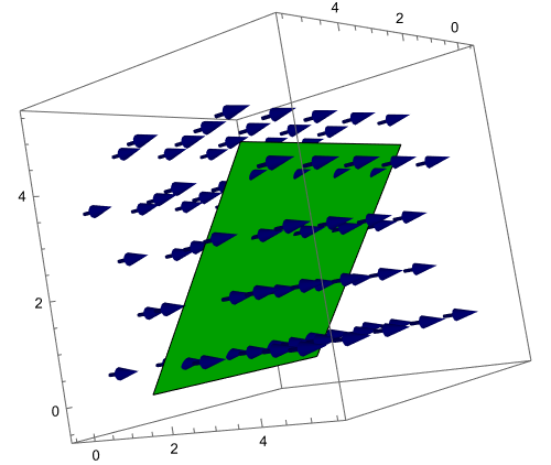
1. In the pictures above, the velocity is given by $\vec F = (0,2,0)$ meters per second and the green surface $S$ is a square with surface area 25 square meters. For each picture above, let's determine the flux of $\vec F$ across $S$.
   1. Explain why the flow rate of $\vec F$ through $S$ for the first image above is 50 cubic meters per second.
   2. Explain why the flow rate of $\vec F$ through $S$ for the second image above is 0 cubic meters per second.
   3. In the third image, the edges of the parallelogram are given by $\vec u = (5,0,0)$ and $\vec v = (0,3,4)$. Compute the flow rate of $\vec F$ through $S$.

In our computations above, we were not concerned about which direction the fluid flowed through the surface. In general, we'll keep track of which direction a fluid flows through a surface, and count flux as negative when the fluid flows the opposite direction. To do this, we pick a unit vector $\hat n$ to the surface, called an orientation of $S$, and decide flux is positive precisely when the vector component of $\vec F$ that is parallel to $\hat n$ is in the same direction as $\hat n$.

4. In the third image above, a normal vector to the surface is $\vec u\times \vec v = (5,0,0)\times (0,3,4) = (0,20,-15)$, which means we can use $\hat n = \frac{\vec u\times \vec v}{|\vec u\times \vec v|} = \frac{1}{5}(0,4,-3)$ as an orientation for $S$. Show that the flux of $\vec F$ across $S$ with the orientation $\hat n$ is $ ( \vec F\cdot \hat n)( \text{Surface Area of $S$ } )$.

The computations above generalize rapidly to provide a method for computing the flux of a vector field $\vec F$ across a surface $S$ in the direction of $\hat n$. For a vector field $\vec F$ and surface $S$ with orientation $\hat n$, we have used $dS$ to represent small bits of surface area. This means a small amount of flux across $S$ is given by $d\text{Flux} = \vec F\cdot \hat n dS$. Summing these, and computing a limit provides the flux as $$\text{Flux}=\Phi = \iint_S \vec F\cdot \hat n dS.$$ Note that because $\hat n$ is a unit normal vector to $S$, then given a parametrization $\vec r(u,v)$ of $S$ for $(u,v)$ in some region $R$, we know $\hat n = \pm \frac{\vec r_u\times \vec r_v}{|\vec r_u\times \vec r_v|} $ while $dS = |\vec r_u\times \vec r_v|dudv$. This means we can simplify the flux integral above to $$\text{Flux}=\Phi = \iint_R \vec F \cdot (\pm\vec r_u\times \vec r_v)dudv,$$ where the $\pm$ sign must be determined based on the orientation of the surface.

2. Let $\vec F = (x^2 + y, y - z, 3 x + 2 z)$ and $S$ be the surface parametrized by $\vec r(u,v) = (3 \cos v,u,3\sin v)$ for $1\leq u\leq 5$ and $0\leq v\leq 2\pi$. Let $\hat n$ be the unit normal to $S$ which points outwards, away from the $y$-axis. Compute the outward flux $\Phi$ of $\vec F$ across $S$. The steps below can serve as a guide.
   • Compute $\vec r_u$ and $\vec r_v$.
   • Compute a normal vector $\vec N = \vec r_u \times \vec r_v$, and decide if $\vec N$ points in the same, or opposite direction, as the orientation $\hat n$. This may require you to draw the surface to visually make that determination.
   • Insert all the known values into $\iint_R \vec F\cdot (\pm\vec r_u\times \vec r_v)dudv$, making sure all variables have been written in terms of $u$ and $v$. Then use software to compute the integral. (I got $72\pi$.)
3. Let $\vec F = (2 y z, x + 3 y, -z^2)$ and $S$ be the surface parametrized by $\vec r(u,v) = (u \cos v, u \sin v, 9 - u^2)$ for $0\leq u\leq 3$ and $0\leq v\leq 2\pi$. Compute the upward ($\hat n$ has positive $z$-component) flux $\Phi$ of $\vec F$ across $S$ in the direction of $\hat n$. The steps above are still the same guide. (I got $-243\pi/2$.)

Task 42.2

For a surface $S$ with parametrization $\vec r(u,v) = (x(u,v),y(u,v),z(u,v))$ for $(u,v)$ in some region $R$, we have shown that surface area is $$S = \iint_S dS = \iint_R |\vec r_u\times\vec r_v|dudv.$$ This means we can compute mass, average values, centroids, centers-of-mass, etc, in a manner similar to what we have already done.

• For a function $f$ defined at points on the surface, the average value is $$\bar f = \frac{\iint_S f dS}{\iint_S dS} = \frac{\iint_R f(u,v) |\vec r_u\times\vec r_v| dudv}{\iint_R |\vec r_u\times\vec r_v| dudv}.$$ Replacing $f$ with $x$, $y$, or $z$ obtains the corresponding coordinate of the centroid of the surface.
• Given a density $\delta$ at points on the surface, the mass of the surface is $$ m = \iint_S dm = \iint_S \delta dS = \iint_R \delta(u,v) |\vec r_u\times\vec r_v| dudv.$$ The center-of-mass is given by $(\bar x, \bar y, \bar z) = \frac{\iint_S (x,y,z) \delta dS}{\iint_S \delta dS}$ which we can write as $$\begin{align*} \bar x &= \frac{\iint_R x(u,v) \delta(u,v) |\vec r_u\times\vec r_v| dudv}{\iint_R \delta(u,v) |\vec r_u\times\vec r_v| dudv},\\ \bar y &= \frac{\iint_R y(u,v) \delta(u,v) |\vec r_u\times\vec r_v| dudv}{\iint_R \delta(u,v) |\vec r_u\times\vec r_v| dudv},\\ \bar z &= \frac{\iint_R z(u,v) \delta(u,v) |\vec r_u\times\vec r_v| dudv}{\iint_R \delta(u,v) |\vec r_u\times\vec r_v| dudv}. \end{align*}$$

Note that there are lots of things going on with each integral. Software will greatly reduce the amount of time needed to set up and compute these integrals. The commands that will be most useful are ParametricPlot3D[], D[], Cross[], Norm[], and Integrate[].

1. Consider the surface $\vec r(u,v) = (3\cos v,3\sin v, u)$ for $1\leq u\leq 5$ and $0\leq v\leq \pi$. Start by drawing the surface. From your picture, state $\bar x$ and $\bar z$. Then set up and compute an integral formula that gives the $y$-coordinate of the centroid.
2. A satellite dish lies along the parametric surface $\vec r(u,v) = (u^2, u\cos v, u\sin v)$ for $0\leq u\leq 2$ and $0\leq v\leq 2\pi$. Start by drawing the surface. The temperature at points on and near the dish is given by $T(x,y,z) = x+z$. Set up and compute an integral formula that gives the average temperature of the satellite dish.
3. The top half of the surface $S$ of a donut (a torus) can be parametrized by $\vec r(u,v) = ((5 - 3 \cos u) \cos v, (5 - 3 \cos u) \sin v, 3 \sin u)$ for $0\leq u\leq \pi$ and $0\leq v\leq 2\pi$. Imagine that someone puts icing on the top of this donut (so creates a surface), but the thickness of the icing is more on the top of the donut than on the sides. While not a perfect way to model this situation, we could use $\delta = kz$ for some constant $k$ as a way to model the surface with varying density. Show that the center-of-mass of the surface $S$ with density function $\delta = kz$ is $(\bar x, \bar y, \bar z) = (0,0,\frac{3\pi}{4})$.

Task 42.3

We've seen all the new notation that we'll encounter for the rest of the semester. This task has us practice using the notation we've learned.

1. Consider the vector field $\vec F = (x,x-z,y+z)$, the surface $S$ parametrized by $\vec r(u,v)=(u^2, u\cos v, u\sin v)$ for $0\leq u\leq 2$ and $0\leq v\leq 2\pi$, and the curve $C$ parametrized by $\vec r(t) = (4,2\cos t, 2\sin t)$ for $0\leq t\leq 2\pi$.
   1. Draw the surface $S$ and curve $C$. How are these two objects related?
   2. Compute $\vec N = \vec r_u\times \vec r_v$ and determine if $\vec N$ points inward toward the $x$-axis, or outwards away from the $x$-axis.
   3. Set up and compute the integral $\ds \int_C Mdx+Ndy+Pdz$, computing the work done by $\vec F$ along $C$.
   4. Set up and compute $\ds \iint_S \vec \nabla \times \vec F\cdot \hat n dS$, computing the flux of the curl of $\vec F$ across $S$ in the direction $\hat n$ outwards away from the $y$-axis.
2. Consider the vector field $\vec F = (x,x-z,y+z)$, the solid domain $D$ that lies inside the sphere $x^2+y^2+z^2=25$, and the surface $S$ parametrized by $\vec r(u,v)=(5\sin v\cos u, 5 \sin v \sin u, 5 \cos v)$ for $0\leq u\leq 2\pi$ and $0\leq v\leq \pi$.
   1. Draw the surface $S$ and domain $D$. How are these two objects related?
   2. Compute $\vec N = \vec r_u\times \vec r_v$ and determine if $\vec N$ points inward toward the domain $D$ or outwards away from the domain $D$.
   3. Set up and compute $\ds \iint_S \vec F\cdot \hat n dS$ for $\hat n$ pointing outwards, away from the solid inside $S$. This computes the outward flux of $\vec F$ across $S$.
   4. Set up and compute $\ds \iiint_D \vec \nabla \cdot \vec F dV$, the triple integral of the divergence of $\vec F$ over the domain $D$.

Task 42.4

Pick some problems related to the topics we are discussing from the Text Book Practice page.

Prep.Day43

There is no new prep. Work on 41.3 and 42.1-3.

Prep.Day44

Task 44.1

What do the curl and divergence of a vector field compute? How do we physically interpret them?

1. Head to the following webpages and read their descriptions.
   • https://mathinsight.org/curl_idea
   • https://mathinsight.org/curl_subtleties
   • https://mathinsight.org/divergence_idea
   • https://mathinsight.org/divergence_subtleties
2. After reading the 4 pages above, head to Wikipedia's article on magnetic fields, see https://en.wikipedia.org/wiki/Magnetic_field. Skim through the article (you do not need to read and comprehend all of it).
   • Are there any new symbols you don't recognize? What are they?
   • Search for the word "divergence" in the text, and read the paragraph(s) where you find it.
   • Search for the word "curl" in the text, and read the paragraph(s) where you find it.
   • Come with questions about anything you would like to discuss.

Task 44.2

As we proceed through the remainder of this unit, we'll find that three types of integrals appear quite often.

• Work integrals: $\ds\int_{C} Mdx+Ndy+Pdz$
• Surface integrals: $\ds \iint_S f(x,y,z) dS$
• Flux integrals: $\ds \iint_S \vec F \cdot \hat n dS$

For each type of integral above, use Mathematica to create a code chunk that you can use to compute each type of integral. This will allow you free yourself from performing tedious computations, letting you focus on bigger picture ideas.

• For the work integral, you can pick the vector field $\vec F(x,y,z)$, parametrization $\vec r(t)$, and bounds for $t$. Feel free to use an example from 42.3.
• For the surface integral, you can pick the surface $S$, function $f(x,y,z)$, parametriztion $\vec r(u,v)$, and bounds for $u$ and $v$. Feel free to use an example from 42.2.
• For the flux integral, you can pick the surface $S$, orientation $\hat n$, parametriztion $\vec r(u,v)$, and bounds for $u$ and $v$. Feel free to use an example from 42.1 or 42.3.

The ReplaceAll[] command in Mathematica will allow you to replace any instance of $x$, $y$, or $z$ with the corresponding value from your parametrization. This allows you to enter the vector field using Cartesian coordinates. Other commands you'll find useful are D[], Cross[], Norm[], Dot[], and Integrate[].

As an example, to dot the vector field $\vec F = (3x+4yz, 2y^2, x-4z)$ with the derivative of the parametrization $\vec r(t) = (3\cos t, 3\sin t, 4 t)$, and then make sure everything is in terms of $t$, we can use the following code.

F = {3 x + 4 y z, 2 y^2, x - 4 z}
r = {3 Cos[t], 3 Sin[t], 4 t}
ReplaceAll[Dot[F, D[r, t]], {x -> r[[1]], y -> r[[2]], z -> r[[3]]}]

(*Or using short cut notation (. for Dot and /. for ReplaceAll)*)
F . D[r, t] /. {x -> r[[1]], y -> r[[2]], z -> r[[3]]}

The notation r[[1]] accesses the first element from r, which is 3 Cos[t].

Task 44.3

Green's theorem connects circulation along a simple closed curve in 2D to an integral along the region inside the curve. The circulation per area (circulation density) is given by $N_x-M_y$ for a 2D vector field. A similar fact is true in 3D, namely if $S$ is a surface with a simple closed curve $C$ that forms the boundary of $S$, then the circulation along $C$ can be computed instead by summing circulation densities (circulation per surface area) along the surface. Given a point $(x,y,z)$ and a unit vector $\hat n$, we calculate the circulation density of $\vec F$ about $\hat n$ at $(x,y,z)$ in a similar manner, as follows.

• We construct a circle $C_a$ of radius $a$ in the plane through $(x,y,z)$ with normal vector $\hat n$.
• We compute the counter-clockwise circulation about $\hat n$, obtaining $\oint_{C_a} Mdx+Ndy+Pdz$.
• We divide by the area $A_a$ inside $C_a$, to obtain a circulation per area.
• The circulation density of $\vec F$ about $\hat n$ at $(x,y,z)$ is the limit $$\lim_{a\to 0}\frac{1}{A_a}\oint_{C_a} Mdx+Ndy+Pdz = \vec \nabla \times \vec F \cdot \hat n.$$

The curl of a vector field provides information about circulation density in every direction (just dot by the direction about which you want to know how things are rotating). Note that for a 2D vector field, we can use the normal vector $\hat n = (0,0,1)$, and then we see that the circulation density for a vector field in 2D is $$(N_z-P_y, P_x-M_z, N_x-M_y) \cdot (0,0,1) = N_x-M_y.$$

We're now ready to state Stokes's theorem.

Let's verify this theorem in some examples.

1. Let $\vec F(x,y,z) = (x+2y, 3x-4z, 2z)$. Consider the surface $S$ parametrized by $\vec r(u,v) = (u\cos v, u\sin v, u^2)$ for $0\leq u\leq 3$ and $0\leq v\leq 2\pi$ with orientation $\hat n$ pointing away from the $z$-axis. The boundary $\partial S$ consists of a single curve $C_1$ parametrized by $\vec r_1(t) = (3\cos t, 3\sin t, 9)$ for $0\leq t\leq 2\pi$.
   1. Draw the surface and curve. Do your best to explain what it means for $\hat n$ and the curve to be oriented compatibly.
   2. Set up and compute the surface integral $\ds \iint_S \vec \nabla \times \vec F \cdot \hat n dS$.
   3. Set up and compute the line integral $\ds \int_{\partial S} Mdx+Ndy+Pdz$. Do you get the same result as the surface integral?
2. Let $\vec F(x,y,z) = (x+2y, 2x+4z, 4y)$. Consider the plane in the first octant with the three vertices $(3,0,0)$, $(0,3,0)$ and $(0,0,3)$. An equation of the plane is $x+y+z=3$, which we can parameterize using $\vec r(u,v) = (u,v,3-u-v)$ for $0\leq u\leq 3$ and $0\leq v\leq 3-u$. The boundary $\partial S$ consists of 3 curves, which we can parameterize using $$\begin{align*} \vec r_1(t) &= (3-3t,3t,0) \quad \text{for} 0\leq t\leq 1,\\ \vec r_2(t) &= (0,3-3t,3t) \quad \text{for} 0\leq t\leq 1,\\ \vec r_3(t) &= (3t,0,3-3t) \quad \text{for} 0\leq t\leq 1. \end{align*}$$
   1. Draw the surface and 3 curves, placing an arrow on the curves to demonstrate the direction of motion.
   2. Compute $\ds \int_{\partial S} Mdx+Ndy+Pdz$ by computing the three line integrals and summing the result.
   3. Compute $\ds \iint_S \vec \nabla \times \vec F \cdot \hat n dS$, using an orientation $\hat n$ that is compatible with the orientation of the curves.

Task 44.4

Pick some problems related to the topics we are discussing from the Text Book Practice page.

Prep.Day45

Task 45.1

We've discussed circulation density and connected it to the curl of a vector field. Let's construct a corresponding analog for flux.

Given a point $(x,y,z)$, we calculate the flux density of $\vec F$ at $(x,y,z)$ as follows.

• We construct a sphere $S_a$ of radius $a$ centered at $(x,y,z)$.
• We compute the outward flux of $\vec F$ across the surface of the sphere, so $\iint_{S_a} \vec F\cdot\hat n dS$.
• We divide by the volume $V_a$ inside $S_a$, to obtain a flux per volume.
• The flux density of $\vec F$ at $(x,y,z)$ is the limit $$\lim_{a\to 0}\frac{1}{V_a}\iint_{S_a}\vec F\cdot\hat n dS = \vec \nabla \cdot \vec F.$$

The divergence of a vector field provides the flux density.

We are now ready to state the divergence theorem.

Let's verify this theorem in some examples.

1. Consider the vector field $\vec F = (x^2, 2 y, x + y + z)$ and sphere of radius 5. We can parameterize the surface $S$ using $\vec r(u,v) = (5 \cos(u)\sin(v),5\sin(u)\sin(v),5\cos(v))$ for $0\leq u\leq 2\pi$ and $0\leq v\leq \pi$. The solid domain $D$ satisfies $\rho\leq 5$ (using spherical coordinates - you'll need appropriate bounds for $\theta$ and $\phi$). Set up and compute both $\iiint_D \vec \nabla \cdot \vec F dV$ and $\iint_{\partial D}\vec F\cdot\hat n dS$, using the outward pointing normal vector $\hat n$. (I got $500\pi$ for both. Pay attention to the direction in which $\vec r_u\times \vec r_v$ points.)
2. Consider the vector field $\vec F = (5x,x-z,y+z+1)$ and solid domain $D$ in space that lies below the paraboloid $z=1-r^2$ (using cylindrical coordinates) and above the $xy$-plane. The boundary of $D$ consists of two surfaces. The top surface is parametrized by $\vec r(u,v) = (u \cos v,u \sin v,1-u^2)$ for $0\leq u\leq 1$ and $0\leq v\leq 2\pi$. The bottom surface is the plane $z=0$, and for this particular problem we can parameterize it using $\vec r(u,v) = (u\cos v,u\sin v,0)$ for $0\leq u\leq 1$ and $0\leq v\leq 2\pi$. Set up and compute both $\iiint_D \vec \nabla \cdot \vec F dV$ and $\iint_{\partial D}\vec F\cdot\hat n dS$, using the outward pointing normal vector $\hat n$. (I got $3\pi$ for both. The flux integral across the top surface is $4\pi$, and across the bottom surface is $-\pi$.)

Task 45.2

Stokes's theorem can be applied when the boundary of a surface consists of disjoint curves. Remember to check if the parametrization associated with each curve is compatible with the orientation on the surface. When not compatible, a simple negative sign can quickly fix any issues.

Let $\vec F = (2x-3y,x^2+2z,4xy)$.

1. Consider the surface $S$ parametrized by $\vec r(u,v) = (u\cos v, u, u \sin v)$ for $1\leq u\leq 3$ and $0\leq v\leq 2\pi$, oriented by $\hat n$ pointing away from the $y$-axis. The boundary $\partial S$ of $S$ is the union of the two disconnected curves $C_1$ with parametrization $\vec r_1(t) = (\cos t, 1, \sin t)$ for $0\leq t\leq 2\pi$ and $C_2$ with parametrization $\vec r_2(t) = (3\cos t, 3, 3\sin t)$ for $0\leq t\leq 2\pi$. Provided the curves are oriented compatibly with $\hat n$, Stokes's theorem states that $$\ds \int_{\partial S} Mdx+Ndy+Pdz = \iint_S \vec \nabla \times \vec F \cdot \hat n dS.$$
   1. Draw the surface and curves.
   2. Compute $\ds \iint_S \vec \nabla \times \vec F \cdot \hat n dS$. (I got $104\pi$.)
   3. Compute $\ds \int_{C_1} Mdx+Ndy+Pdz$ and $\ds \int_{C_2} Mdx+Ndy+Pdz$, using the parametrizations provided.
   4. Explain how to combine the results of the previous computations to obtain $\ds \int_{\partial S} Mdx+Ndy+Pdz$.
2. Now instead let $S$ be half of the surface above, parametrized by $\vec r(u,v) = (u\cos v, u, u \sin v)$ for $1\leq u\leq 3$ and $0\leq v\leq \pi$. The boundary of $S$ now consists of 4 connected curves, two arcs and two straight lines. One arc has parametrization $\vec r_1(t) = (\cos t, 1, \sin t)$ for $0\leq t\leq \pi$. One of the straight lines has parametrization $\vec r_2(t) = (t, t, 0)$ for $1\leq t\leq 3$.
   1. Compute $\ds \iint_S \vec \nabla \times \vec F \cdot \hat n dS$ (change the bounds of what you did in the previous part).
   2. Give parametrizations for the other two curves that make up $\partial S$.
   3. Compute $\ds \int_{C} Mdx+Ndy+Pdz$ for each of the 4 curves in $\partial S$. (You'll end up with $6+2\pi$, $54+54\pi$, $14/3$, and $86/3$, all of which could be negative instead of positive, based on your parametrization.)
   4. Explain how to combine the results of the previous computations to obtain $\ds \int_{\partial S} Mdx+Ndy+Pdz$.

Task 45.3

At this point, we've seen all the topics for the semester, and just need to make sure we practice them all. If you haven't yet, please create blocks of Mathematica code that will help you quickly compute work, surface integrals, and flux integrals, as well as quickly see $\vec r_u\times \vec r_v$ so you can make decisions about in which direction this normal vector points. I'll add more problems for later days. If you want more to work on before then, head to OpenStax and tackle any of the problems in 6.6, 6.7, or 6.8.

Task 45.4

Pick some problems related to the topics we are discussing from the Text Book Practice page.

Prep.Day46

Continue working on the tasks from Day 45 and Day 44.

Prep.Day47

Task 47.1

Consider the vector field $\vec F = \frac{ (x,y,z) }{ (x^2+y^2+z^2) ^{3/2}}$. This vector field is directly proportional to gravitational and electric fields. In this task, we will show that flux of this field across any closed surface that contains the origin is $4\pi$, while the flux across any surface that does not contain the origin is zero.

1. Show that the divergence of $\vec F$ is 0, provided $(x,y,z)\neq(0,0,0)$. You can to this by hand, or with software, or find the solution somewhere online (one of the links in 44.1 has the work).
2. Consider the surface $S$ which is a sphere of radius $a$ (so $x^2+y^2+z^2=a^2$). Compute the outward flux of $\vec F$ across $S$, and show that you get $$\Phi = \iint_S \vec F\cdot \hat n dS = 4\pi.$$ In particular, notice that the answer does not depend on the radius of the sphere. There are multiple ways to do this. One option is to obtain a parametrization of the surface (look back at previous problems to get a parametrization) and then set up and compute the integral directly. Another is to reason out geometrically what $\hat n$ must equal because we're on a sphere of radius $a$, and then replace $x^2+y^2+z^2$ with $a^2$ in many places.
3. Let $S$ be any closed surface which does not contain $(0,0,0)$ on the surface, or inside the surface. Explain why $\iint_S \vec F\cdot \hat n dS =0$
4. Let $S$ be any closed surface which does contain $(0,0,0)$ inside the surface. Explain why $\iint_S \vec F\cdot \hat n dS =4\pi$. (Start by picking a small radius $a$ so that the sphere $x^2+y^2+z^2=a^2$ lies entirely inside $S$.)

Task 47.2

Let $D$ be the solid region in space that lies above the cone $z^2=x^2+y^2$ and below the paraboloid $z=6-x^2-y^2$. In cylindrical coordinates, the domain $D$ lies above the cone $z=r$ and below the paraboloid $z=6-r^2$. Let $\vec F = (x^2, 4y+z, z-x+3)$. Verify the divergence theorem for this solid region. A parametrization for the cone is $\vec r(u,v) = (u\cos v, u\sin v, u)$ for $0\leq u\leq 2$ and $0\leq v\leq 2\pi$. A parametrization for the parabaloid is $\vec r(u,v) = (u\cos v, u\sin v, 6-u^2)$ for $0\leq u\leq 2$ and $0\leq v\leq 2\pi$.

• Compute $\iint_S \vec F\cdot \hat n dS$ across the cone, making sure you have an outward pointing normal vector.
• Compute $\iint_S \vec F\cdot \hat n dS$ across the paraboloid, making sure you have an outward pointing normal vector.
• Compute $\iiint_D \vec \nabla \cdot \vec F dV$, and show how to combine the results of the previous computations to get the same value.

In my work above, I ended up seeing the values $-20\pi/3$, $60\pi$, and $160\pi/3$.

Task 47.3

Pick a problem from OpenStax from 6.7 or 6.8, where it asks you to verify either Stokes' or the Divergence theorem, and complete it.

Task 47.4

Pick some problems related to the topics we are discussing from the Text Book Practice page.

Prep.Day48

Learning Target Checkoff

A learning target quiz will appear in I-Learn. Complete and submit the quiz before the due date.

Prep.Day49

No prep for today.

Prep.Day50

Learning target quiz. No class.