
- I-Learn, Class Pictures, Learning Targets, Text Book Practice
- Prep Tasks: Unit 1 - Motion, Unit 2 - Derivatives, Unit 3 - Integration, Unit 4 - Vector Calculus
We still have Tasks 12.2 and 12.3 to discuss in class.
Day 12 - Prep
Task 12.1
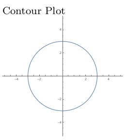
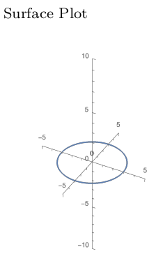
A computer chip has been disconnected from electricity and sitting in cold storage for quite some time. The chip is connected to power, and a few moments later the temperature (in Celsius) at various points $(x,y)$ on the chip is measured. From these measurements, statistics is used to create a temperature function $z=f(x,y)$ to model the temperature at any point on the chip. Suppose that this chip's temperature function is given by the equation $z=f(x,y)=9-x^2-y^2$. (This could just as easily have been the elevation of a rover at a point $(x,y)$ on a hill.) We'll be creating both a 2D contour plot (topographical map) and 3D surface plot of this function in this task.
The points in the plane with temperature $f(x,y)=0$ satisfy $0=9-x^2-y^2$, or equivalently $x^2+y^2=9$. These points lie on a circle of radius 3, so we can draw that circle in the $xy$-plane (the start of our 2D contour plot) and also in 3D by plotting a circle of radius 3 at height $z=0$ (the start of our 3D surface plot). These two plots are shown below.
- What is the temperature at $(0,0)$, $(1,2)$, and $(-4,3)$?
- Which points in the plane have temperature $z=5$? Add this contour (level curve) to your 2D contour plot. Then at height $z=5$, add the same curve to the 3D surface plot.
- Repeat the above for $z=8$, $z=9$, and $z=1$. What's wrong with letting $z=10$?
- Letting $y = 0$ provides a vertical cross section of the surface. This is the curve $z = 9-x^2-0^2$. This curve cannot be drawn on the contour plot, but can be added to your 3D surface plot. Add that curve, and then add the curve given by letting $x=0$.
- Describe the 3D surface that you created with your plot. Add any extra features to your 3D surface plot to convey the 3D image you constructed. You can use the Mathematica file ContourSurfaceGradient.nb to check your work.
- For the function $f(x,y) = x^2-y$, construct a 2D contour plot and 3D surface plot.
Task 12.2
Suppose that an explosion occurs at the origin $(0,0,0)$. Heat from the explosion starts to radiate outwards. Suppose that a few moments after the explosion, the temperature at any point in space is given by $w=T(x,y,z)=100-x^2-y^2-z^2.$
- Which points in space have a temperature of 99? To answer this, replace $T(x,y,z)$ by $99$ to get $99=100-x^2-y^2-z^2$. Use algebra to simplify this to $x^2+y^2+z^2=1$. Draw this object.
- Which points in space have a temperature of 96? of 84? Draw the surfaces.
- What is the temperature at $(3,0,-4)$? Draw the set of points that have this same temperature.
- The 4 surfaces you drew above are called level surfaces. If you walk along a level surface, what happens to your temperature?
- When we compute a level surface of a function $w = f(x,y,z)$, which variable do we make constant? When we compute a level curve of a function $z=f(x,y)$, which variable do we make constant?
- Consider now the function $w=f(x,y,z)=x^2+z^2$. This function has an input $y$, but notice that changing the input $y$ does not change the output of the function.
- Draw a graph of the level surface $w=4$. [When $y=0$ you can draw one curve. When $y=1$, you draw the same curve. When $y=2$, again you draw the same curve. This kind of graph we call a cylinder, and is important in manufacturing where you extrude an object through a hole.]
- Graph the level surface $9=x^2+z^2$ (so $w=9$), and $w=16$.
You can use the Mathematica file ContourSurfaceGradient.nb to check your work.
Task 12.3
Suppose the elevation $z$ of terrain near a rover is given by the formula $z=f(x,y) = x^2+3xy$.
- Suppose that $x$ and $y$ are both functions of $t$, and then use implicit differentiation to compute $\dfrac{dz}{dt}$. Write your answer in the form $$\frac{dz}{dt} = (?)\frac{dx}{dt}+(?)\frac{dy}{dt}.$$
- The differential of $z$ (or differential of $f$ as $z=f(x,y)$) is obtained by multiplying both sides above by $dt$. Verify that $dz = (2x+3y)dx+3xdy$.
- Write the differential of $f$ as the dot product $$df = (?,?)\cdot(dx,dy).$$
When we write the differential of a function $f(x,y)$ in the form $df = M dx +N dy$, we call $M$ the partial derivative of $f$ with respect to $x$, written $f_x$ or $\frac{\partial f}{\partial x}$ or $D_x f$, and we call $N$ the partial derivative of $f$ with respect to $y$, written $f_y$ or $\frac{\partial f}{\partial y}$ or $D_y f$. The vector $(f_x,f_y)$ we call the gradient of $f$, written as $\vec\nabla f$, which means the differential of $f$ is always $$df = \vec \nabla f \cdot (dx,dy) = (f_x, f_y)\cdot (dx,dy) = f_xdx+f_ydy.$$ Similar definitions hold for functions of more variables.
- For the function $f(x,y)=3x^2+2xy$, compute the differential $df$ (in terms of $x$, $y$, $dx$, $dy$), the partial derivatives $f_x$ and $f_y$, and the gradient $\vec \nabla f(x,y)$.
- For the function $g(r,s,t)=r^2s^3+4rt^2$ compute the differential $dg$ (in terms of $r$, $s$, $t$, $dr$, $ds$, $dt$), the partial derivatives $g_r$ and $\frac{\partial g}{\partial s}$ and $D_tg$, and the gradient $\vec \nabla g(r,s,t)$.
Task 12.4
The last problem for prep each day will point to relevant problems from OpenStax. Spend 30 minutes working on problems from the sections below.
- section 4.1 exercises 14-29, 30-32, 39-41, 42-47, 48-52, 53-58
Day 14 - Prep
We'll spend today revisiting the prep for Day 13. You can jump ahead to day 15 if you want to get ahead. Click to view the Day 13 prep.
Day 13 - Prep
Task 13.1
For the function $f(x,y) = 9-x^2-y^2$, we can compute the differential $df = -2xdx-2ydy$, the partial derivatives $f_x = -2x$ and $f_y=-2y$, along with the gradient $\vec \nabla f(x,y) = (-2x,-2y)$. Notice that the gradient is a vector field, so at the point $(x,y)$ we can draw the vector $(-2x,-2y)$.
- Construct a plot of the vector field $\vec \nabla f(x,y) = (-2x,-2y)$.
- Add to your vector field plot a contour plot of $f(x,y) = 9-x^2-y^2$ (we constructed a contour plot for the function in a previous Task).
- What relationships do you see between the vectors from the gradient plot, and the level curves from your contour plot.
For the function $f(x,y) = x^2-y$, we can compute the differential $df = 2xdx-1dy$, the partial derivatives $f_x = 2x$ and $f_y=-1$, along with the gradient $\vec \nabla f(x,y) = (2x,-1)$. Again, notice that the gradient is a vector field, so at the point $(x,y)$ we can draw the vector $(2x,-1)$.
- Construct a plot of the vector field $\vec \nabla f(x,y) = (2x,-1)$.
- Add to your vector field plot a contour plot of $f(x,y) = x^2-y$ (we constructed a contour plot for the function in a previous Task).
- What relationships do you see between the vectors from the gradient plot, and the level curves from your contour plot.
You can use the Mathematica file ContourSurfaceGradient.nb to check your work.
Task 13.2
Suppose the Mars rover Curiosity is currently on a hill, and its position is at the center of the map on the left below. Zooming in on the rover's position yields the map on the right below (the color legend applies to the graph on the right).
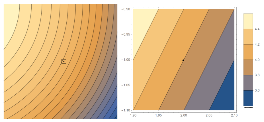
The contours in the graph to the right each represent a change in height of 0.2 units. The bounds for the graph are $1.9\leq x\leq 2.1$ and $-1.1\leq y\leq -0.9$. For simplicity of computations, let's assume the $x$, $y$ and $z$ axes use the same units. The rover is currently located at the point $(2,-1)$, shown as a dot.
The rover can head in many directions. In this problem we'll estimate the slope in several directions. For example, if the rover follows the vector $(0,1)$, heads north, then it has to move a distance (run) of $\Delta y = 0.1$ units to hit the next contour, resulting in a change in height of $\Delta z = +0.2$ units. This means the slope in the $(0,1)$ direction is $$\ds\frac{\text{rise}}{\text{run}} = \frac{\Delta z}{\text{distance moved in $xy$ plane}} = \frac{+0.2}{0.1} = 2.$$
- Estimate the slope if the rover heads east, following $(1,0)$.
- If the rover heads south, following $(0,-1)$, estimate the slope.
- If the rover follows the direction $(1,1)$ (so northeast), what distance must the rover travel to hit the next contour? Use this to estimate the slope in the $(1,1)$ direction.
- Estimate the slope in the $(1,2)$ direction.
Rather than starting with a contour plot and using it to visually estimate slopes, let's start with a function of the form $z=f(x,y)$ and use it to compute slopes. Suppose the elevation $z$ of terrain near the rover is given by the formula $z=f(x,y) = x^2+3xy$, and the rover is currently at $P=(2,-1)$.
- Compute the differential $dz$ and write it in the form $dz = (?)dx+(?)dy$. Then evaluate $dz$ at the rover's location $P=(2,-1)$. [Check: Did you get $dz = (1)dx+(6)dy$?]
- If the rover follows the direction $(dx,dy)$, explain why the slope is $\frac{dz}{\sqrt{(dx)^2+(dy)^2}}$.
- Estimate the slope if the rover heads east, following $(dx,dy)=(1,0)$. Then estimate the slope if the rover heads north, following $(dx,dy)=(0,1)$. What do these values have to do with the partial derivatives of $f$?
- Estimate the slope in the $(1,1)$ direction and then the $(1,2)$ direction.
Task 13.3
The volume of a right circular cylinder is $V(r,h)= \pi r^2 h$.
- If we think of $h$ as a constant, so that $V(r)$ is only a function of $r$, then compute $\frac{dV}{dr}$.
- If instead we think of $r$ as a constant, so that $V(h)$ is only a function of $h$, then compute $\frac{dV}{dh}$.
- Compute the differential of $V(r,h)$, and then state the gradient $\vec \nabla V(r,h)$ along with the partial derivatives $\frac{\partial V}{\partial r}$ and $\frac{\partial V}{\partial h}$.
- If we know $r=3$ and $h=4$, and we know that $r$ could increase by $dr=0.1$ and $h$ could increase by about $dh=0.2$, then use differentials to estimate how much $V$ will increase.
Notice that we were able to compute the partial derivatives above, without ever needing to compute the differential first. We obtain $\frac{\partial V}{\partial r}$ by imagining that every variable other than $r$ was a constant, and then computing the regular derivative.
- The volume of a box is given by $f(x,y,z)=xyz$. Without computing the differential, compute $\frac{\partial f}{\partial x}$, $\frac{\partial f}{\partial y}$, and $\frac{\partial f}{\partial z}$.
- Now compute the differential $df$ (use implicit differentiation if needed) and verify that the partial derivatives you computed before actually show up in the differential $df$.
- If the current measurements are $x=2$, $y=3$, and $z=5$, and we know that expected tolerances are $dx=.01$, $dy=.02$, and $dz=.03$, then estimate the change in volume.
Task 13.4
The last problem for prep each day will point to relevant problems from OpenStax. Spend 30 minutes working on problems from the sections below.
- section 4.3, exercises 118-131
Day 14 - In class
Brain Gains (Rapid Recall, Jivin' Generation)

- For the function $w=f(x,y,z) = x^2+z^2$, draw the level surface corresponding to $w=9$.
- For the function $w=f(x,y,z) = x^2+z^2$, draw the level surface corresponding to $w=16$.
- Compute the gradient of $f(x,y,z) = x^2+z^2$.
- At the point $P = (3,0,0)$, draw the gradient $\vec \nabla f(P)$. Then repeat this at $P = (0,0,3)$ and $P = (-4,0,0)$.
Group Problems
- Compute $f_x$ and $\frac{\partial f}{\partial y}$ for each of the following (try to do it without computing $df$ first).
- $f(x,y) = x^2y$
- $f(x,y) = 3xy+4y^2$
- $f(x,y) = \sin(xy^2)$
- Consider the function $z=f(x,y) = x-y^2$.
- Compute $\vec \nabla f$.
- Construct a 2D contour plot by hand. So pick several values for $z$ and plot the resulting curves. If you end up with lots of horizontal lines in the $xy$-plane, you're doing this correctly. Write the height on each horizontal line you draw.
- Construct a 3D surface plot by hand.
- Remember that the gradient is a vector field. At a few points in your contour plot, add the gradient vector.
- Check your work with ContourSurfaceGradient.nb.
- A rover is located on a hill whose elevation is given by $z=f(x,y) = 3x^2+2xy+4y^2$.
- Compute the differential $dz$, and state the gradient $\vec \nabla f$.
- State $\dfrac{\partial f}{\partial x}$ and $f_y$.
- State the differential at the point $P=(1,1)$ (the spot where the rover currently resides) [Check: $dz = 8dx+10dy$].
- What is the slope of the hill at $P=(x,y)=(1,1)$ in the direction $(dx,dy)=(1,0)$?
- What is the slope of the hill at $P=(1,1)$ in the direction $(0,1)$?
- What is the slope of the hill at $P=(1,1)$ in the direction $(3,4)$? [Check: $\frac{64}{5}$. The rise is $dz = 64$, with a run of $5$.]
- Let $g(x,y) =x^2y$.
- Give $g_x$ and $\dfrac{\partial g}{\partial y}$. Then state $\vec \nabla g$.
- Find the slope of $g$ at $P=(3,1)$ in the direction $(-3,2)$.
- Find the slope of $g$ at $P=(3,1)$ in the direction $(2,-5)$.
Day 15 - Prep
Every time we compute a differential $df = f_xdx+ f_ydy$, we're following a pattern that shows up so often that it's given a name (linear combination). At some point you may take a linear algebra course where you'll focus quite a bit on linear combinations, and quickly adopt matrices to help speed up the process of writing linear combinations.
Given $n$ vectors $\vec v_1, \vec v_2,\cdots,\vec v_n$ and $n$ scalars $c_1, c_2, \cdots, c_n$ the linear combination of these vectors using these scalars is the sum $$\sum_{i=1}^n c_1 \vec v_i = c_1\vec v_1+c_2\vec v_2+\cdots+c_n\vec v_n.$$ Matrix notation and products were invented to organize linear combinations into a visually appealing compact form. We place each vector in the column of a matrix, and then place the corresponding scalars into a single column vector after the matrix. The linear combination above, in matrix form, becomes the matrix product $$c_1\vec v_1+c_2\vec v_2+\cdots+c_n\vec v_n = \begin{bmatrix} \begin{pmatrix}\\\vec v_1\\ \ \end{pmatrix} &\begin{pmatrix}\\\vec v_2\\ \ \end{pmatrix} &\cdots &\begin{pmatrix}\\\vec v_n\\ \ \end{pmatrix} \end{bmatrix} \begin{pmatrix}c_1\\c_2\\\vdots\\c_n\end{pmatrix}.$$
The derivative (or total derivative) of a function is a matrix whose columns are the partial derivatives of the function. The partial derivatives we insert into the columns of the matrix in the same order in which the variables are listed for the function. Some examples follow.
- For the function $f(x)$, the derivative is $Df(x) = \begin{bmatrix}f_x\end{bmatrix} =\begin{bmatrix}\frac{df}{dx}\end{bmatrix}$, with differential $df = f_xdx$.
- For the function $f(x,y)$, the derivative is $Df(x,y) = \begin{bmatrix}f_x&f_y\end{bmatrix}$, with differential $df = f_xdx+f_ydy$.
- For the function $f(r,s,t)$, the derivative is $Df(r,s,t) = \begin{bmatrix}f_r&f_s&f_t\end{bmatrix}$, with differential $df = f_rdr+f_sds+f_tdt$.
- For the function $\vec r(u,v)$, the derivative is $D\vec r(u,v) = \begin{bmatrix}\vec r_u&\vec r_v\end{bmatrix}$, with differential $d\vec r = \vec r_udu+\vec r_vdv$.
Task 15.1
Let's practice using the definitions above. For each function below, (a) compute and label all relevant partial derivatives. Then (b) write the differential $df$ as a linear combination of the partial derivatives. Then (c) write $df$ as a matrix product. Finish by (d) stating the total derivative $Df$ of the function.
- $f(x,y)=x^2y$ [Clearly label all 4 things you were asked to find, namely (a) all partials, (b) $df$ as a linear combination, (c) $df$ as a matrix product, and (d) the derivative $Df$.]
- $f(x,y)=x^2+2xy+3y^2$
- $f(x,y,z)=3xz-x^2y$
Task 15.2
The gradient of a function $f(x,y)$ is itself a function. When we compute the partial derivatives of the gradient, we obtain vectors instead of numbers. This task has you examine the differential, partials, and derivative of the gradient of a function. We'll soon see that the derivative of the gradient is precisely the key to classifying maximums and minimums of a function.
The function $f(x,y) = x^2+3xy+2y^2$ has the gradient $\vec \nabla f = (2x+3y,3x+4y)$. This is the vector field $$\vec F = (2x+3y,3x+4y).$$
- Find the differential $d\vec F$ and write it as the linear combination $$d\vec F = \begin{pmatrix}?\\?\end{pmatrix}dx+\begin{pmatrix}?\\?\end{pmatrix}dy.$$
- Rewrite the above differential as a matrix product, so fill in the blanks below. $$d\vec F = \begin{pmatrix}?&?\\?&?\end{pmatrix}\begin{pmatrix}?\\?\end{pmatrix}.$$
- Clearly label the two partial derivatives $\frac{\partial \vec F}{\partial x}$ and $\vec F_y$.
- State the total derivative $D\vec F(x,y)$ (it should be a 2 by 2 matrix). [Note: We also write the derivative of the gradient as $D^2f(x,y)$, or $D\vec\nabla f(x,y)$, and call the resulting matrix the Hessian of $f$. Some people use the notation $\vec \nabla ^2 f$ for the Hessian, though this notation also gets use for the Laplacian $\vec \nabla \cdot (\vec \nabla f)$, which is a very different quantity.]
- The function $f(x,y) = xy^2$ has gradient $\vec F = (y^2, 2xy)$. Repeat the above to obtain the differential of $\vec F$ (as a linear combination, and in matrix form), the partials of $\vec F$, and the derivative $D\vec F(x,y)$.
Task 15.3
Suppose a rover moves along the level curve of a function $f(x,y)$ following the path $\vec r(t)=(x,y)$. An example of such a scenario is shown below (note that lighter colors correspond to greater outputs of $f(x,y)$. )
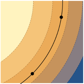
Label the dots $A$ and $B$ (it doesn't matter which you label $A$ or $B$). Our goal is to prove that the gradient of $f$ is normal to level curves.
- At each dot in the picture on the right, draw a vector that represents a possible option for $\ds\frac{d\vec r}{dt} = \left(\frac{dx}{dt},\frac{dy}{dt}\right)$.
- Suppose $\vec r(0)=A$ and $\vec r(1)=B$. If we know that $f(\vec r(0)) = 7$, then what is $f(\vec r(1))$? Explain.
- As the rover moves along $\vec r(t)$, how much does $f$ change? Use this to give a value for $\ds\frac{df}{dt}$?
- Explain why $\vec \nabla f$ and $\ds\frac{d\vec r}{dt}$ are orthogonal at any point along the level curve. (Hint: Add $dt$ to the denominators of the the differential $df = f_xdx+f_ydy$ , and then write the differential as a dot product. Since we are on a level curve, we know the value of $\ds\frac{df}{dt}$.)
- At point $A$, draw a vector that points in the same direction as $\vec \nabla f(A)$. Use your work above to explain why the gradient of $f$ must be normal to the level curve.
Task 15.4
The last problem for prep each day will point to relevant problems from OpenStax. Spend 30 minutes working on problems from the sections below.
- Return to any of the previous day's OpenStax problems to locate extra practice.
|
Sun |
Mon |
Tue |
Wed |
Thu |
Fri |
Sat |