Derivatives

Task 1

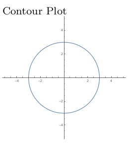
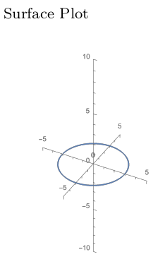
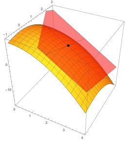
A computer chip has been disconnected from electricity and sitting in cold storage for quite some time. The chip is connected to power, and a few moments later the temperature (in Celsius) at various points $(x,y)$ on the chip is measured. From these measurements, statistics is used to create a temperature function $z=f(x,y)$ to model the temperature at any point on the chip. Suppose that this chip's temperature function is given by the equation $z=f(x,y)=9-x^2-y^2$. (This could just as easily have been the elevation of a rover at a point $(x,y)$ on a hill.) We'll be creating both a 2D contour plot (topographical map) and 3D surface plot of this function in this task.

The points in the plane with temperature $f(x,y)=0$ satisfy $0=9-x^2-y^2$, or equivalently $x^2+y^2=9$. These points lie on a circle of radius 3, so we can draw that circle in the $xy$-plane (the start of our 2D contour plot) and also in 3D by plotting a circle of radius 3 at height $z=0$ (the start of our 3D surface plot). These two plots are shown below.

1. What is the temperature at $(0,0)$, $(1,2)$, and $(-4,3)$?
2. Which points in the plane have temperature $z=5$? Add this contour (level curve) to your 2D contour plot. Then at height $z=5$, add the same curve to the 3D surface plot.
3. Repeat the above for $z=8$, $z=9$, and $z=1$. What's wrong with letting $z=10$?
4. Letting $y = 0$ provides a vertical cross section of the surface. This is the curve $z = 9-x^2-0^2$. This curve cannot be drawn on the contour plot, but can be added to your 3D surface plot. Add that curve, and then add the curve given by letting $x=0$.
5. Describe the 3D surface that you created with your plot. Add any extra features to your 3D surface plot to convey the 3D image you constructed. Check your work with the following Mathematica code.

   f[x_, y_] := 9 - x^2 - y^2
   ContourPlot[f[x, y], {x, -2, 2}, {y, -2, 2}]
   Plot3D[f[x, y], {x, -2, 2}, {y, -2, 2}]
   Plot3D[f[x, y], {x, -2, 2}, {y, -2, 2}, MeshFunctions -> {#3 &}]
   

6. For the function $f(x,y) = x^2-y$, construct a 2D contour plot and 3D surface plot, first by hand, and then with Mathematica.

Task 2

Suppose that an explosion occurs at the origin $(0,0,0)$. Heat from the explosion starts to radiate outwards. Suppose that a few moments after the explosion, the temperature at any point in space is given by $w=T(x,y,z)=100-x^2-y^2-z^2.$

1. Which points in space have a temperature of 99? To answer this, replace $T(x,y,z)$ by $99$ to get $99=100-x^2-y^2-z^2$. Use algebra to simplify this to $x^2+y^2+z^2=1$. Draw this object.
2. Which points in space have a temperature of 96? of 84? Draw the surfaces.
3. What is the temperature at $(3,0,-4)$? Draw the set of points that have this same temperature.
4. Modify the code below to redraw, with Mathematica, each of the surfaces you previously drew.

   f[x_, y_, z_] := x^2 + y^2 - z^2
   ContourPlot3D[f[x, y, z] == 2, {x, -5, 5}, {y, -5, 5}, {z, -5, 5}]
   

5. The 4 surfaces you drew above are called level surfaces. If you walk along a level surface, what happens to your temperature?
6. When we compute a level surface of a function $w = f(x,y,z)$, which variable do we make constant? When we compute a level curve of a function $z=f(x,y)$, which variable do we make constant?
7. Consider now the function $w=f(x,y,z)=x^2+z^2$. This function has an input $y$, but notice that changing the input $y$ does not change the output of the function.
   • Draw a graph of the level surface $w=4$. [When $y=0$ you can draw one curve. When $y=1$, you draw the same curve. When $y=2$, again you draw the same curve. This kind of graph we call a cylinder, and is important in manufacturing where you extrude an object through a hole.]
   • Graph the level surface $9=x^2+z^2$ (so $w=9$), and $w=16$.
   • Rather than drawing one surface at a time, Mathematica can draw all the surfaces at once, using the Contours option. Modify the code below to draw the three level surfaces in the same plot.

     f[x_, y_, z_] := x^2 + y^2 - z^2
     ContourPlot3D[f[x, y, z], {x, -5, 5}, {y, -5, 5}, {z, -5, 5}, 
      Contours -> {-10, 0, 2, 20}, ContourStyle -> Opacity[0.5]]
     

Task 3

Suppose the elevation $z$ of terrain near a rover is given by the formula $z=f(x,y) = x^2+3xy$.

1. Suppose that $x$ and $y$ are both functions of $t$, and then use implicit differentiation to compute $\dfrac{dz}{dt}$. Write your answer in the form $$\frac{dz}{dt} = (?)\frac{dx}{dt}+(?)\frac{dy}{dt}.$$ Check you work with Mathematica, using the code below.

   f[x_, y_] := x^2 + 3 x y
   z[t_] := f[x[t], y[t]]
   z'[t]
   

2. The differential of $z$ (or differential of $f$ as $z=f(x,y)$) is obtained by multiplying both sides above by $dt$. Verify that $dz = (2x+3y)dx+3xdy$.
3. Write the differential of $f$ as the dot product $$df = (?,?)\cdot(dx,dy).$$

When we write the differential of a function $f(x,y)$ in the form $df = M dx +N dy$, we call $M$ the partial derivative of $f$ with respect to $x$, written $f_x$ or $\frac{\partial f}{\partial x}$ or $D_x f$, and we call $N$ the partial derivative of $f$ with respect to $y$, written $f_y$ or $\frac{\partial f}{\partial y}$ or $D_y f$. The vector $(f_x,f_y)$ we call the gradient of $f$, written as $\vec\nabla f$, which means the differential of $f$ is always $$df = \vec \nabla f \cdot (dx,dy) = (f_x, f_y)\cdot (dx,dy) = f_xdx+f_ydy.$$ Similar definitions hold for functions of more variables.

f[x_, y_] := x^2 + 3 x y
D[f[x, y], x]
D[f[x, y], y]
D[f[x, y], {{x, y}}]

Note that prime notation is no longer useful when there are two or more variables.

4. For the function $f(x,y)=3x^2+2xy$, compute the differential $df$ (in terms of $x$, $y$, $dx$, $dy$), the partial derivatives $f_x$ and $f_y$, and the gradient $\vec \nabla f(x,y)$. Use Mathematica to check that your partials and gradient are correct.
5. For the function $g(r,s,t)=r^2s^3+4rt^2$ compute the differential $dg$ (in terms of $r$, $s$, $t$, $dr$, $ds$, $dt$), the partial derivatives $g_r$ and $\frac{\partial g}{\partial s}$ and $D_tg$, and the gradient $\vec \nabla g(r,s,t)$. Use Mathematica to check that your partials and gradient are correct.

Self Check

I'll occasionally add relevant problems from OpenStax. As needed, spend a few minutes working on some exercises below. If you get stuck on a prep task, feel free to bring a solution to one of the textbook exercises to share.

• section 4.1 exercises 14-29, 30-32, 39-41, 42-47, 48-52, 53-58

Task 4

For the function $f(x,y) = 9-x^2-y^2$, we can compute the differential $df = -2xdx-2ydy$, the partial derivatives $f_x = -2x$ and $f_y=-2y$, along with the gradient $\vec \nabla f(x,y) = (-2x,-2y)$. Notice that the gradient is a vector field, so at the point $(x,y)$ we can draw the vector $(-2x,-2y)$.

1. Construct a plot of the vector field $\vec \nabla f(x,y) = (-2x,-2y)$.
2. Add to your vector field plot a contour plot of $f(x,y) = 9-x^2-y^2$.
3. What relationships do you see between the vectors from the gradient plot, and the level curves from your contour plot.
4. Construct the plots above with Mathematica. You'll need VectorPlot[] and ContourPlot[] to create the plots, and Show[] to get both plots in the same figure.

For the function $f(x,y) = x^2-y$, we can compute the differential $df = 2xdx-1dy$, the partial derivatives $f_x = 2x$ and $f_y=-1$, along with the gradient $\vec \nabla f(x,y) = (2x,-1)$. Again, notice that the gradient is a vector field, so at the point $(x,y)$ we can draw the vector $(2x,-1)$.

4. Construct a plot of the vector field $\vec \nabla f(x,y) = (2x,-1)$.
5. Add to your vector field plot a contour plot of $f(x,y) = x^2-y$ (we constructed a contour plot for the function in a previous Task).
6. What relationships do you see between the vectors from the gradient plot, and the level curves from your contour plot.
7. Create the plots with software, if you haven't already.

Task 5

Suppose the Mars rover Curiosity is currently on a hill, and its position is at the center of the map on the left below. Zooming in on the rover's position yields the map on the right below (the color legend applies to the graph on the right).

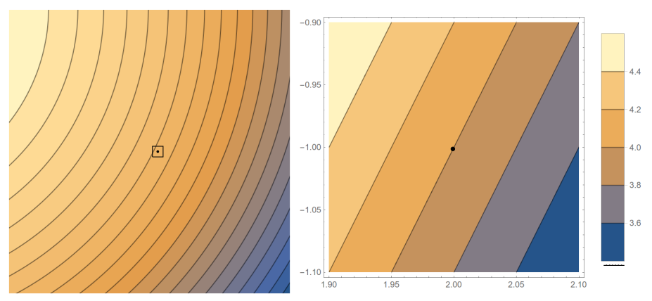
The contours in the graph to the right each represent a change in height of 0.2 units. The bounds for the graph are $1.9\leq x\leq 2.1$ and $-1.1\leq y\leq -0.9$. For simplicity of computations, let's assume the $x$, $y$ and $z$ axes use the same units. The rover is currently located at the point $(2,-1)$, shown as a dot.

The rover can head in many directions. In this problem we'll estimate the slope in several directions. For example, if the rover follows the vector $(0,1)$, heads north, then it has to move a distance (run) of $\Delta y = 0.1$ units to hit the next contour, resulting in a change in height of $\Delta z = +0.2$ units. This means the slope in the $(0,1)$ direction is $$\ds\frac{\text{rise}}{\text{run}} = \frac{\Delta z}{\text{distance moved in $xy$ plane}} = \frac{+0.2}{0.1} = 2.$$

1. Estimate the slope if the rover heads east, following $(1,0)$.
2. If the rover heads south, following $(0,-1)$, estimate the slope.
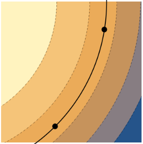
3. If the rover follows the direction $(1,1)$ (so northeast), what distance must the rover travel to hit the next contour? Use this to estimate the slope in the $(1,1)$ direction.
4. Estimate the slope in the $(1,2)$ direction.

Rather than starting with a contour plot and using it to visually estimate slopes, let's start with a function of the form $z=f(x,y)$ and use it to compute slopes. Suppose the elevation $z$ of terrain near the rover is given by the formula $z=f(x,y) = x^2+3xy$, and the rover is currently at $P=(2,-1)$.

5. Compute the differential $dz$ and write it in the form $dz = (?)dx+(?)dy$. Then evaluate $dz$ at the rover's location $P=(2,-1)$. [Check: Did you get $dz = (1)dx+(6)dy$?]
6. If the rover follows the direction $(dx,dy)$, explain why the slope is $\frac{dz}{\sqrt{(dx)^2+(dy)^2}}$.
7. Estimate the slope if the rover heads east, following $(dx,dy)=(1,0)$. Then estimate the slope if the rover heads north, following $(dx,dy)=(0,1)$. What do these values have to do with the partial derivatives of $f$?
8. Estimate the slope in the $(1,1)$ direction and then the $(1,2)$ direction.

Task 6

The volume of a right circular cylinder is $V(r,h)= \pi r^2 h$.

1. If we think of $h$ as a constant, so that $V(r)$ is only a function of $r$, then compute $\frac{dV}{dr}$.
2. If instead we think of $r$ as a constant, so that $V(h)$ is only a function of $h$, then compute $\frac{dV}{dh}$.
3. Compute the differential of $V(r,h)$, and then state the gradient $\vec \nabla V(r,h)$ along with the partial derivatives $\frac{\partial V}{\partial r}$ and $\frac{\partial V}{\partial h}$. Check your answers using Mathematica's D[] command.
4. If we know $r=3$ and $h=4$, and we know that $r$ could increase by $dr=0.1$ and $h$ could increase by about $dh=0.2$, then use differentials to estimate how much $V$ will increase.

Notice that we were able to compute the partial derivatives above, without ever needing to compute the differential first. We obtain $\frac{\partial V}{\partial r}$ by imagining that every variable other than $r$ was a constant, and then computing the regular derivative.

5. The volume of a box is given by $f(x,y,z)=xyz$. Without computing the differential, and without software, compute $\frac{\partial f}{\partial x}$, $\frac{\partial f}{\partial y}$, and $\frac{\partial f}{\partial z}$.
6. Now compute the differential $df$ without software (use implicit differentiation if needed) and verify that the partial derivatives you computed before actually show up in the differential $df$.
7. Check your computations for the partial derivatives are correct, using software.
8. If the current measurements are $x=2$, $y=3$, and $z=5$, and we know that expected tolerances are $dx=.01$, $dy=.02$, and $dz=.03$, then estimate the change in volume.

Self Check

I'll occasionally add relevant problems from OpenStax. As needed, spend a few minutes working on some exercises below. If you get stuck on a prep task, feel free to bring a solution to one of the textbook exercises to share.

• section 4.3, exercises 118-131

Every time we compute a differential $df = f_xdx+ f_ydy$, we're following a pattern that shows up so often that it's given a name (linear combination). At some point you may take a linear algebra course where you'll focus quite a bit on linear combinations, and quickly adopt matrices to help speed up the process of writing linear combinations.

Task 7

Let's practice using the definitions above. For each function below, (a) compute and label all relevant partial derivatives. Then (b) write the differential $df$ as a linear combination of the partial derivatives. Then (c) write $df$ as a matrix product. Finish by (d) stating the total derivative $Df$ of the function.

1. $f(x,y)=x^2y$ [Clearly label all 4 things you were asked to find, namely (a) all partials, (b) $df$ as a linear combination, (c) $df$ as a matrix product, and (d) the derivative $Df$.]
2. $f(x,y)=x^2+2xy+3y^2$
3. $f(x,y,z)=3xz-x^2y$

Task 8

The gradient of a function $f(x,y)$ is itself a function. When we compute the partial derivatives of the gradient, we obtain vectors instead of numbers. This task has you examine the differential, partials, and derivative of the gradient of a function. We'll soon see that the derivative of the gradient is precisely the key to classifying maximums and minimums of a function.

The function $f(x,y) = x^2+3xy+2y^2$ has the gradient $\vec \nabla f = (2x+3y,3x+4y)$. This is the vector field $$\vec F = (2x+3y,3x+4y).$$

1. Find the differential $d\vec F$ and write it as the linear combination $$d\vec F = \begin{pmatrix}?\\?\end{pmatrix}dx+\begin{pmatrix}?\\?\end{pmatrix}dy.$$
2. Rewrite the above differential as a matrix product, so fill in the blanks below. $$d\vec F = \begin{pmatrix}?&?\\?&?\end{pmatrix}\begin{pmatrix}?\\?\end{pmatrix}.$$
3. Clearly label the two partial derivatives $\frac{\partial \vec F}{\partial x}$ and $\vec F_y$.
4. State the total derivative $D\vec F(x,y)$ (it should be a 2 by 2 matrix). [Note: We also write the derivative of the gradient as $D^2f(x,y)$, or $D\vec\nabla f(x,y)$, and call the resulting matrix the Hessian of $f$. Some people use the notation $\vec \nabla ^2 f$ for the Hessian, though this notation also gets use for the Laplacian $\vec \nabla \cdot (\vec \nabla f)$, which is a very different quantity.]
5. Not much changes, notationally, when computing partials and derivatives of a vector field. Use the code below to check that your partials and total derivative are correct.

   F[x_, y_] := {2 x + 3 y, 3 x + 4 y}
   D[F[x, y], x]
   D[F[x, y], y]
   D[F[x, y], {{x, y}}]
   D[F[x, y], {{x, y}}] // MatrixForm
   (*MatrixForm just creates a pretty version of the matrix for humans.*)
   

6. The function $f(x,y) = xy^2$ has gradient $\vec F = (y^2, 2xy)$. Repeat the above to obtain the differential of $\vec F$ (as a linear combination, and in matrix form), the partials of $\vec F$, and the derivative $D\vec F(x,y)$. Finish by checking your work with Mathematica.

Task 9

Suppose a rover moves along the level curve of a function $f(x,y)$ following the path $\vec r(t)=(x,y)$. An example of such a scenario is shown below (note that lighter colors correspond to greater outputs of $f(x,y)$. )

Label the dots $A$ and $B$ (it doesn't matter which you label $A$ or $B$). Our goal is to prove that the gradient of $f$ is normal to level curves.

1. At each dot in the picture on the right, draw a vector that represents a possible option for $\ds\frac{d\vec r}{dt} = \left(\frac{dx}{dt},\frac{dy}{dt}\right)$.
2. Suppose $\vec r(0)=A$ and $\vec r(1)=B$. If we know that $f(\vec r(0)) = 7$, then what is $f(\vec r(1))$? Explain.
3. As the rover moves along $\vec r(t)$, how much does $f$ change? Use this to give a value for $\ds\frac{df}{dt}$?
4. Explain why $\vec \nabla f$ and $\ds\frac{d\vec r}{dt}$ are orthogonal at any point along the level curve. (Hint: Add $dt$ to the denominators of the the differential $df = f_xdx+f_ydy$ , and then write the differential as a dot product. Since we are on a level curve, we know the value of $\ds\frac{df}{dt}$.)
5. At point $A$, draw a vector that points in the same direction as $\vec \nabla f(A)$. Use your work above to explain why the gradient of $f$ must be normal to the level curve.

Task 10

We'll focus this task on making sure we understand how differentials can help us approximate changes in a function.

A forest ranger needs to estimate the height of a tree. The ranger stands 50 feet from the base of tree and measures the angle of elevation to the top of the tree to be about 60$^\circ$.

1. If this angle of 60$^\circ$ is correct, then what is the height of the tree? Explain in general why the height of the tree is $h(\theta) = 50 \tan \theta$.
2. Compute the differential $dh$ in terms of $\theta$ and $d\theta$.
3. The ranger's angle measurement is mostly likely off by some amount. If the error in the ranger's measurement could be as much as $d\theta = 5^\circ$ (so $\frac{5\pi}{180}$ radians), then use differentials to estimate how large the error in the height could be (so compute $dh$). If your answer here is quite large (much larger than the height of the tree), then look back at your work and see if using radians instead of degrees makes a difference. Why does it? Feel free to ask in class.
4. Compute the height if the angle were exactly 65 instead of 60. What's the actual difference between these two heights?

The US mint creates coins that are roughly a cylindrical shape, with volume $V = \pi r^2h$. Unfortunately, not every coin is exactly the same size, and small errors in $r$ (given by $dr$) and small errors in $h$ (given by $dh$), affect the amount of material needed to mint these coins.

5. Compute $dV$ to give an approximate for the change in volume given by the errors $dr$ and $dh$.
6. The radius of a coin is much larger than the height. Will an error in the radius, or an error in the height, cause a larger change in volume? Explain using your differentials.
7. A soda can company has a cylindrical shape that instead has a large $h$ with small $r$. Will an error in the radius, or an error in the height, cause a larger change in volume in this situation.

Task 11

Suppose that a rover is located at point $P=(x,y)$ on a hill whose elevation is given by $z=f(x,y)$. The rover will be moving in the direction parallel to $\vec u$.

1. Explain why the slope of the hill at $P$ in the direction $\vec u = (dx,dy)$ is given by $$\frac{dz}{\sqrt{(dx)^2+(dy)^2}}.$$
2. Prove that this slope can be written, using gradients, as $$\vec \nabla f(P) \cdot \frac{\vec u}{|\vec u|}.$$
3. Use the above fact to compute the slope of a hill given by $f(x,y) = x^2+3xy$ at $P=(2,-1)$ in the direction $\vec u = (3,4)$. (We call this the directional derivative of $f$ at $P$ in the direction $\vec u$, written $D_{\vec u}f(P)$.)
4. The code below computes the directional derivative. Check your work, using this code.

   D[x^2 + 3 x y, {{x, y}}].{3,4}/Norm[{3,4}] /. {x -> 2, y-> -1}
   

   Then try adapting the code to allow you to type in a function $f(x,y)$, a point $P$, and a direction $\vec u$, separate from the directional derivative computation. Here's a start.

   f[x_, y_] := x^2 + 3 x y
   P = {2, -1}
   u = {3, 4}
   

The directional derivative of $f$ in the direction of the vector $\vec u$ at a point $P$ is defined to be $$D_{\vec u} f(P)=\vec \nabla f(P) \cdot \frac{\vec u}{|\vec u|}.$$ We can simplify the above to just $D_{\vec u} f(P)=\vec \nabla f(P) \cdot \hat u$ if $\hat u$ is a unit vector. We dot the gradient of $f$ at $P$ with a unit vector in the direction of $\vec u$.

5. Show that the partial derivative of $f$ with respect to $x$ is precisely the directional derivative of $f$ in the $(1,0)$ direction. [Hint: Compute, symbolically, the dot product $\vec \nabla f \cdot (1,0)$.]
6. Show that the partial derivative of $f$ with respect to $y$ is precisely the directional derivative of $f$ in the $(0,1)$ direction.

Please watch this short 2 part video that discusses the gradient a bit more, and how you can connect the gradient to the slope in various directions.

• https://www.youtube.com/watch?v=8g2bGLjTLEI&list=PLyLfbaRW-ocMjPvsB_NjXxZDHXSFXUS_A&index=1

Task 12

In first semester calculus, differential notation is $dy=f' dx$. At $x=c$, the tangent line passes through the point $P=(c,f(c))$. If $Q=(x,y)$ is any other point on the line, then the vector $\vec {PQ} = (x-c,y-f(c))$ tells us that when $dx=x-c$ we have $dy=y-f(c)$. Substitution give us an equation for the tangent line tangent line as $$\underbrace{y-f(c)}_{dy}={f'(c)}\underbrace{(x-c)}_{dx}.$$ This equation tells us that a change in the output ($y-f(c)$) equals the derivative times a change in the input ($x-c$). In this task, we'll repeat this process to obtain an equation of a tangent plane to a function $f(x,y)$, where differential notation gives $$dz = \frac{\partial f}{\partial x}dx+\frac{\partial f}{\partial y}dy.$$

Consider the function $z=f(x,y)=9-x^2-y^2$. We'll be finding an equation of the tangent plane to $f$ at $(x,y)=(2,1)$. Here is a surface plot along with the tangent plane at $(2,1,f(2,1))$, together with a contour plot.

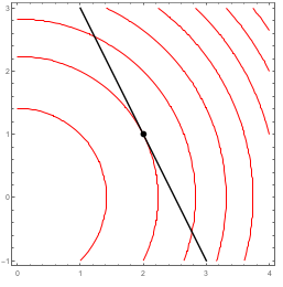
1. Compute the partial derivatives $f_x$ and $f_y$, and the differential $dz$. At the point $(x,y) = (2,1)$, evaluate the partial derivatives and the function $z=f(x,y)$.
2. One point on the tangent plane to the surface at $(2,1)$ is the point $P=(2,1,f(2,1))$. Let $Q=(x,y,z)$ be another point on this plane. Use the vector $\vec{PQ}$ to obtain $dz$ when $dx = x-2$ and $dy = y-1$.
3. We'd like an equation of the tangent plane to $f(x,y)$ when $x=2$ and $y=1$. Differential notation tells us that $$\underbrace{z-?}_{dz}=(-4)\underbrace{(x-?)}_{dx}+(?)\underbrace{(y-?)}_{dy}.$$ Fill in the blanks to get an equation of the tangent plane.
4. Rewrite the equation you got in the form $A(x-a)+B(y-b)+C(z-c)=0$ and state a normal vector to the plane.
5. The level curve of $f$ that passes through $(2,1)$ has no change in height, so $dz=0$. Use this fact to give an equation of the tangent line to this level curve at $(2,1)$.

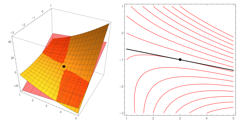
Now let $z=f(x,y)=x^2+4xy+y^2$. At the point $P=(x,y)=(3,-1)$, we'll give an equation of the tangent plane to the surface and an equation of the tangent line to the level curve of $f$ that passes through this point.

6. Give an equation of the tangent plane at $P=(x,y)=(3,-1)$. [Hint: Find $f_x$, $f_y$, $dx$, $dy$, and then $dz$, all at $(x,y)=(3,-1)$. Then substitute, as done above.]
7. The level curve of $f$ that passes through $P$ is a curve in the plane. Give an equation of the tangent line to this curve at $P$. [Hint: Since we're on a level curve, what does $dz$ equal? The equation is almost identical to the previous part, with one minor change based on what $dz$ equals.]

The tangent plane and tangent line you just found are shown below.

Task 13

A rover moves on a hill where elevation is given by $z=f(x,y)=9-x^2-y^2$. The rover's path is parametrized by $\vec r(t)=(2\cos t, 3\sin t)$.

1. At time $t=0$, what is the rover's position $\vec r(0)$, and what is the elevation $f(\vec r(0))$ at that position? Then find the positions and elevations at $t=\pi/2$, $t=\pi$, and $t=3\pi/2$ as well.
2. In the $xy$-plane, draw the rover's path for $t\in [0,2\pi]$. Then, on the same 2D graph, include a contour plot of the elevation function $f$. Include the level curves that pass through the points in part 1. Along each level curve drawn, state the elevation of the curve. [If you end up with an ellipse and several concentric circles, then you've done this right. As a challenge, try to do this in Mathematica.]
3. As the rover follows its elliptical path, the elevation is rising and falling. At which $t$ does the elevation reach a maximum? A minimum? Explain, using your graph.
4. As the rover moves past the point at $t=\pi/4$, is the elevation increasing or decreasing? In other words, is $\dfrac{df}{dt}$ positive or negative at $t=\pi/4$? Use your graph to explain.

Notice above that we wanted $\frac{df}{dt}$, the rate of change of elevation with respect to time, even though the function $f(x,y)$ does not explicitly have $t$ as an input. The proper notation would be $\frac{d(f\circ r)}{dt}$, but this is so cumbersome that it's generally avoided. The notation $\frac{df}{dt}$ requires the reader to infer from context that $x$ and $y$ depend on $t$.

5. At the point $\vec r(t)$, we'd like a formula for the elevation $f(\vec r(t))$. What is the elevation of the rover at any time $t$? [In $f(x,y)$, replace $x$ and $y$ with what they are in terms of $t$.]
6. Compute $df/dt$ (the derivative as you did in first-semester calculus).

Let's repeat the above, but first compute differentials before substitution. For reference, we let $f(x,y)=9-x^2-y^2$ and $(x,y)=\vec r(t)=(2\cos t, 3\sin t)$.

7. Compute the differential $df$ in terms of $x$, $y$, $dx$, and $dy$.
8. Compute $dx$ and $dy$ in terms of $t$ and $dt$.
9. Use substitution to write $df$ in terms of $t$ and $dt$. Then divide by $dt$ to obtain $\frac{df}{dt}$. Did you get the same answer as the previous part?
10. Use your work above to state both $\vec\nabla f(x,y)$ and $\frac{d\vec r}{dt}$. Show that $\frac{df}{dt} = \vec\nabla f(x,y)\cdot \frac{d\vec r}{dt}$.

Task 14

Consider the functions $f(x,y,z) = xy^2z^3$ and $g(x,y)=x\cos(xy)$.

1. First compute $\vec \nabla f$. Then compute $f_{xy}$ and $\frac{\partial^2 f}{\partial z\partial y}$. Explain how you got these. End by computing the entire second derivative $D\vec\nabla f(x,y,z)$ (it is a 3 by 3 matrix with all 9 second partials placed inside).
2. Compute $g_x$ and then $g_{xy}$. Then compute $g_y$ followed by $g_{yx}$.
3. Now let $f(x,y)=3xy^3+e^{x}.$ Compute the four second partials $$\ds \frac{\partial^2 f}{ \partial x^2},\quad \ds\frac{\partial^2 f}{\partial y \partial x},\quad \ds\frac{\partial^2 f}{\partial y^2}, \quad \text{ and }\ds\frac{\partial^2 f}{\partial x \partial y}.$$
4. For $f(x,y)=x^2\sin(y)+y^3$, compute both $f_{xy}$ and $f_{yx}$.
5. Make a conjecture about a relationship between $f_{xy}$ and $f_{yx}$. Then use your conjecture to quickly compute $f_{xy}$ if $$f(x,y)=3xy^2+\tan^{2}(\cos(x)) (x^{49}+x)^{1000}.$$
6. Repeat all the computations above in Mathematica.

Task 15

In the first printed calculus textbooks, there was no mention of the chain rule. This is because differentials were extremely common notation, and the chain rule, when working with differentials, is simply substitution. In this task, we'll develop some rules for how to compute derivatives when functions depend on other functions (so composite functions).

1. Suppose that $f(x,y,z) = ax+by+cz$, and $x=mt$, $y=nt$, and $z = pt$, for some constants $a,b,c,m,n,p$. Compute the differentials $df$, $dx$, $dy$, and $dz$. Then use substitution to obtain the differential of $f$ in terms of $t$ and $dt$. Finish by stating $\frac{df}{dt}$.
   • Check your answer with the Mathematica code below (come with questions if you're not sure how to read the output).

     ClearAll[f, x, y, z, t]
     D[f[x[t], y[t], z[t]], t]
     
2. Suppose now that $g$ is a function of $x$ and $y$, but $x$ and $y$ are functions of $u$, $v$, and $w$. This means, by definition of the differential and partial derivatives, that $dg = g_xdx+g_ydy$, along with $dx = x_udu+x_vdv+x_wdw$ and $dy = y_udu+y_vdv+y_wdw$. Substitution gives $$\begin{align*} dg &= g_xdx+g_ydy\\ &= g_x(x_udu+x_vdv+x_wdw)+g_y(y_udu+y_vdv+y_wdw)\\ &= (?)du+(?)dv+ (?)dw. \end{align*}$$ Fill in the question marks above, and then use your answer to state the three partials $\dfrac{\partial g}{\partial u}$, $g_v$, and $D_w g$.
   • Check your answer with the Mathematica code below.

     ClearAll[g, x, y, z, u, v, w]
     D[g[x[u, v, w], y[u, v, w]], u]
     D[g[x[u, v, w], y[u, v, w]], v]
     D[g[x[u, v, w], y[u, v, w]], w]
     
3. Consider the function $h(x,y,z)$, where $x$, $y$, and $z$ are functions of $r$ and $\theta$. State the differentials of $h$, $x$, $y$, and $z$, and then use substitution to prove that $$\dfrac{\partial h}{\partial r} = \dfrac{\partial h}{\partial x}\dfrac{\partial x}{\partial r} +\dfrac{\partial h}{\partial y}\dfrac{\partial y}{\partial r} +\dfrac{\partial h}{\partial z}\dfrac{\partial z}{\partial r}.$$ Obtain a similar formula for $\dfrac{\partial h}{\partial \theta}$.
   • Create Mathematica code that will compute these partial derivatives for you.

Ask me in class how this relates to matrix multiplication.

Task 16

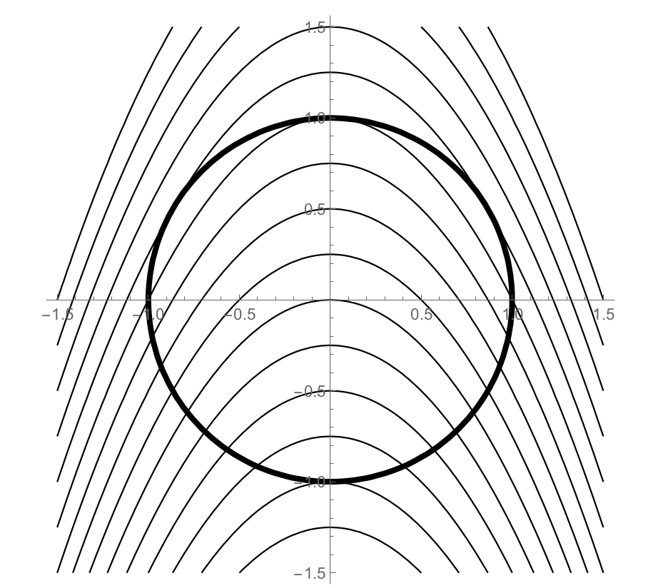
Suppose a rover travels around the circle $g(x,y)=x^2+y^2=1$. The elevation of the surrounding terrain is $f(x,y) = x^2+y+4$. The plot below shows the rover's path (the constraint $g(x,y)=1$), placed on the same grid as a contour plot of the elevation (the function $f(x,y)$ we wish to optimize).

The code below generates the plot above.

f[x_, y_] := x^2 + y + 4
g[x_, y_] := x^2 + y^2
c = 1
p1 = ContourPlot[f[x, y], {x, -1.5, 1.5}, {y, -1.5, 1.5}, 
   ContourShading -> None, Contours -> Table[i, {i, 2, 6, 0.25}], 
   Axes -> True, Frame -> None];
p2 = ContourPlot[g[x, y] == c, {x, -1.5, 1.5}, {y, -1.5, 1.5}, 
   ContourStyle -> {Black, Thick}];
Show[p1, p2]

Each level curve above represents a difference in elevation of 0.25 m. Our goal is to find the maximum and minimum elevation reached by the rover as it travels around the circle. We will optimize $f(x,y)$ subject to the constraint $g(x,y)=1$.

1. Label each level curve with its elevation. Print this page, or copy the curves down on your paper.
   • At which $(x,y)$ point does the rover encounter the minimum elevation? What is the minimum elevation? Explain, using the plot.
   • Suppose the rover is currently at the point $(0,1)$ on its circular path. As the rover moves left, will the elevation rise or fall? What if the rover moves right? Is $(0,1)$ the location of a local maximum or local minimum?
   • On your graph, place a dot(s) where the rover reaches a maximum elevation. What is the maximum elevation? Explain.
2. Rather than visually inspecting level curves, let's examine the gradients $\vec \nabla f$ and $\vec \nabla g$ to see how these gradients compare at maximums and minimums.
   • On the graph above, draw $\vec \nabla f$ at lots of places on your contour plot.
   • At lots of points on the circle, with a different color, draw $\vec \nabla g$.
   • Make sure you draw both gradients at all the points corresponding to local maxes and mins.
   • The following Mathematica code adds the gradients of $f$ and $g$ at all points (not just points on the level curves you drew). Run this code to verify your work by hand.

     gradf = D[f[x, y], {{x, y}}]
     gradg = D[g[x, y], {{x, y}}]
     p3 = VectorPlot[gradf, {x, -1.5, 1.5}, {y, -1.5, 1.5}, 
        VectorStyle -> Red, VectorColorFunction -> None, 
        VectorMarkers -> Placed["Arrow", "Start"], VectorSizes -> Small];
     p4 = VectorPlot[gradg, {x, -1.5, 1.5}, {y, -1.5, 1.5}, 
        VectorStyle -> Green, VectorColorFunction -> None, 
        VectorMarkers -> Placed["Arrow", "Start"], VectorSizes -> Tiny];
     Show[p1, p2, p3, p4]
     

3. At the local maximums and minimums, Lagrange noticed that $\vec \nabla f = \lambda \vec \nabla g$.
   • How would you interpret the equation $\vec \nabla f = \lambda \vec \nabla g$?
   • Compute $\vec \nabla f$ and $\vec \nabla g$.
   • Explain why the system of equations $\vec \nabla f = \lambda \vec \nabla g$ and $g(x,y)=c$ is equivalent to the system of equations $$2x = \lambda 2x,\quad 1=\lambda 2y,\quad x^2+y^2=1.$$
   • Solve the system of equations above to obtain 4 ordered pairs $(x,y)$.
   • Check your work with Mathematica's Solve[] command.

     f[x_, y_] := x^2 + y + 4
     g[x_, y_] := x^2 + y^2
     c = 1
     gradf = D[f[x, y], {{x, y}}]
     gradg = D[g[x, y], {{x, y}}]
     Solve[{gradf == \[Lambda] gradg, g[x, y] == c}, {x, y, \[Lambda]}]
     

   • At each ordered pair, find the elevation. What is the maximum elevation obtained, and where does it occur? What is the minimum elevation obtained, and where does it occur?

Task 17

This task will mostly involve reading through some definitions and an example, with a short example at the end.

A = {{6, 2}, {2, 3}}
A // MatrixForm
Eigenvalues[A]

The identity matrix $I$ is a square matrix with 1's on the diagonal and zeros everywhere else, so in 2D we have $I = \begin{pmatrix} 1&0\\0&1 \end{pmatrix}$. To find the eigenvalues, we rewrite $A\vec x = \lambda\vec x$ in the form $A\vec x -\lambda\vec x=\vec 0$ or $A\vec x -\lambda I \vec x=\vec 0$, which becomes $(A-\lambda I) =\vec 0.$ We need to find the values $\lambda$ so that $\left(\begin{bmatrix} a&c\\b&d\end{bmatrix}-\lambda \begin{bmatrix} 1&0\\0&1 \end{bmatrix} \right)\begin{pmatrix}x\\y\end{pmatrix} =\begin{pmatrix}0\\0\end{pmatrix} \quad\text{or}\quad \begin{bmatrix} a-\lambda &c\\b&d-\lambda \end{bmatrix}\begin{pmatrix}x\\y\end{pmatrix} =\begin{pmatrix}0\\0\end{pmatrix}.$ A linear algebra course will show that $\lambda$ satisfies $$(a-\lambda)(d-\lambda)-bc=0.$$

Let's look at an example. Consider $f(x,y)=x^2-2x+xy+y^2$. The gradient is $\vec \nabla f(x,y)=(2x-2+y,x+2y)$. The critical points of $f$ occur where the gradient is zero. We need to solve the system $2x-2+y=0$ and $x+2y=0$, which is equivalent to solving $2x+y=2$ and $x+2y=0$. Double the second equation, and then subtract it from the first to obtain $0x-3y=2$, or $y=-2/3$. The second equation says that $x=-2y$, or that $x=4/3$. So the only critical point is $(4/3,-2/3)$.

The second derivatives is $ D^2f = \begin{bmatrix}2&1 \\1&2\end{bmatrix}.$ The second derivative is constant, so $D^2 f(4/3,-2/3)$ is the same as $D^2f(x,y)$. (In general, the critical point may affect your matrix.) To find the eigenvalues we solve $$(2-\lambda)(2-\lambda)-(1)(1)=0.$$ Expanding the left hand side gives $4-4\lambda + \lambda^2 -1 = 0$. Simplifying and factoring gives us $\lambda^2-4\lambda +3 = (\lambda-3)(\lambda -1) = 0$. The eigenvalues are $\lambda = 1$ and $\lambda=3$. Since both numbers are positive, we know the gradient points outwards away from the critical point. The critical point $(4/3,-2/3)$ corresponds to a local minimum of the function. The local minimum is the output $f(4/3,-2/3) = (4/3)^2-2(4/3)+(4/3)(-2/3)+(-2/3)^2$.

Mathematica will find the critical values (by solving a system), and then find the eigenvalues of the second derivative at each critical point, using the code below.

f[x_, y_] := x^2 - 2 x + x y + y^2

(*Find the critical points - when is the gradient zero?*)
gradf = D[f[x, y], {{x, y}}]
cpts = Solve[gradf == {0, 0}, {x, y}]

(*Compute the second derivative, evaluate it at the first (and only) critical point, and then find the corresponding eigenvalues.*)
hessianf = D[gradf, {{x, y}}]
hessianf /. cpts[[1]] // MatrixForm
Eigenvalues[hessianf /. cpts[[1]]]

(*With more critical points, just increment the 1 as needed.*)

Let's try this process on our own. Consider the function $f(x,y)=x^2+4xy+y^2$.

1. Find the critical points of $f$ by finding when $Df(x,y)$ is the zero matrix.
2. Find the eigenvalues of $D^2f$ at any critical points.
3. Label each critical point as a local maximum, local minimum, or saddle point, and state the value of $f$ at the critical point.
4. Use Mathematica (adapt the code above) to verify that you obtained the correct values.

Task 18

Consider the function $f(x,y)=x^3-3x+y^2-4y$.

1. Find the critical points of $f$ by finding when $Df(x,y)$ is the zero matrix. [Hint: You should obtain two critical points.]
2. Find the eigenvalues of $D^2f$ at any critical points. [Hint: First compute $D^2f$. Since there are two critical points, evaluate the second derivative at each point to obtain 2 different matrices. Then find the eigenvalues of each matrix.]
3. Label each critical point as a local maximum, local minimum, or saddle point, and state the value of $f$ at the critical point.
4. Adapt the Mathematica code given previously to perform all these computations for you.
5. Now use Mathematica to construct a 2D contour plot and 3D surface plot of the function to visually verify that your solution is correct. Choose bounds for your plots so that the critical points are clearly visible.

Task 19

Let's now return to a Lagrange multiplier problem, where we have a constraint that limits the values over which we want to optimize a function. Consider the curve $xy^2=54$.

1. Start by drawing the curve.

The distance from each point on this curve to the origin is a function that must have a minimum value. We will find a point $(a,b)$ on the curve that is closest to the origin.

The first step to any Lagrange multiplier problem is to identify the function $f(x,y)$ that we wish to maximize or minimize, and then then identify the constraint and write it in the form $g(x,y) = c$. The distance from $(x,y)$ to the origin is $d(x,y) = \sqrt{(x-0)^2+(y-0)^2}=\sqrt{x^2+y^2}.$ This is the function we wish to minimize. The square root on this function will complicate computations later on. Because the square root function is increasing, note that $h(x,y) = x^2+y^2$ will have its minimum value at the same place as $d(x,y)$. Because of this, we can simplify our work and use $f(x,y)=x^2+y^2$ as the function we wish to minimize.

2. What's the constant $c$ and function $g$ so that our constraint can be written in the form $g(x,y)=c$?
3. Solve the system $\vec \nabla f = \lambda \vec \nabla g$ and $g=c$.
   • After computing the gradients, state the 3 equations that form the system we must solve, and then solve it.
   • Note that in this problem, the number $\lambda$ is not an eigenvalue, rather it is a multiplier that helps us know if $\vec \nabla f$ and $\vec \nabla g$ lie on the same line (are parallel or antiparallel, i.e. "Is one gradient a multiple of the other?".)
   • Use Mathematica to solve this system, to verify that you have the correct solution. When you solve this system in Mathematica, you'll obtain 6 solutions, of which 4 of them contain complex numbers (use //N to numerically approximate the solutions if needed, and you'll see many solutions contain an imaginary component).
4. State the $(x,y)$ coordinates on the curve $xy^2=54$ that are closest to the origin.
5. How does the problem above change if we want to find the point on the curve that is closest to $(3,4)$? Solving the corresponding system of equations by hand will not be simple, but we can use Mathematica quickly answer this question, once we state $f$, $g$, and $c$. You will need to numerically approximate the solution that Mathematica gives (type //N at the end of a line of code to numerically approximate the output). Show how to adapt the code to obtain the solutions $(x,y) = (3.11122,4.16612)$.
   • Mathematica will also gives you the solution $(x,y) = (5.22184, -3.21577)$. Why is this NOT a point on the curve that is closest to $(3,4)$?

Task 20

Consider the function $f(x,y,z) = -x^2+y^2+z^2$.

1. Start by using the ContourPlot3D[] command in Mathematica to draw several level surfaces of this function.

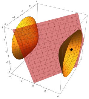
The level surface which passes through the point $(3,2,-1)$ is shown below, along with the tangent plane to the surface through the point $(3,2,-1)$. This surface is called a hyperboloid of two sheets.

2. Use the differential $$df = f_xdx+f_ydy+f_zdz \quad\text{or}\quad df=\vec\nabla f(a,b,c)\cdot(dx,dy,dz) . $$ to give an equation of the tangent plane to this surface at the point $(3,2,-1)$. [Hint: Start by explaining why $df=0$. Then we have $dx=x-3$, $dy=y-?$, and $dz =?$. Don't forget to evaluate the partials at the correct point.]
3. Suppose the function $f(x,y,z) = -x^2+y^2+z^2$ gives the temperature (in Celcius) at points in space near some object (located at the origin), with $x,y,z$ values given in meters. Compute the temperature at $(3,2,-1)$, and then use differentials to approximate the temperature at $(3.01,1.98, -0.98)$. [What are $dx$, $dy$, and $dz$?]
4. Compute the directional derivative of $f(x,y,z) = -x^2+y^2+z^2$ at the point $(3,2,-1)$ in the direction $(1, -2, 2)$. What are the units of $D_{ (1, -2, 2) }f(3,2,-1)$?
5. What similarities, and what differences, do you see in the three questions above?

Task 21

This task will have you practice using the second derivative test to locate maxima, minima, and/or saddle points for function $f(x,y)$ of two variables.

1. Consider the function $f(x,y)=x^3-3x+y^2-4y$.
   1. Find the critical points of $f$ by finding when $Df(x,y)$ is the zero matrix.
   2. Find the eigenvalues of $D^2f$ at any critical points. [Hint: First compute $D^2f$. Since there are two critical points, evaluate the second derivative at each point to obtain 2 different matrices. Then find the eigenvalues of each matrix.]
   3. Label each critical point as a local maximum, local minimum, or saddle point, and state the value of $f$ at the critical point.
   4. Check your work with Mathematica.
2. Consider the function $f(x,y) = 6x^2-2x^3+3y^2+6xy$. The function has two critical points $(0,0)$ and $(1,-1)$. At each of these points, evaluate the second derivative and then find the corresponding eigenvalues. Use these eigenvalues to classify each critical point as the location of a local maximum, local minimum, or saddle point. Finish by checking your work with Mathematica.

Task 22

To use Lagrange Multipliers, we must (1) identify the function $f(x,y)$ to be optimized along with the constant $c$ and function $g$ in the constraint $g(x,y)=c$, (2) write the system of equations that results from $\vec \nabla f = \lambda \vec \nabla g$ and $g(x,y)=c$, (3) solve this system, and (4) determine which points correspond to maxes and which to mins. The third step, solving a system of equations, can become extremely difficult quite quickly, but luckily modern software can help facilitate this part of the process. Check all solutions with Mathematica (code for doing so can be found in previous tasks).

1. Let $f(x,y) = 20 x + 2 y^2$. Use Lagrange multipliers to identify the location of any extreme values of $f$ along the line $100=4x+8y$. Complete this by hand, and then check your work with software.
2. A rover travels along a circle of radius 5, centered at the origin. The elevation of the surrounding hill is give by $z = 4x^2-4xy+y^2$. What are the highest and lowest elevations reached by the rover? [If the system to solve is too brutal, then use software to help you.]

Task 23

Suppose a rover is located at a point $P$ on a hill whose elevation is given by $z=f(x,y)$. Recall that the directional derivative of $\vec f$ at $P$ in the direction $\vec u$ is the dot product $D_{\vec u} f(P)=\vec \nabla f(P)\cdot \frac{\vec u}{|\vec u|}.$ Also recall that we can compute dot products using the law of cosines $\vec \nabla f(P)\cdot \vec u= |\vec \nabla f(P)| |\vec u|\cos\theta,$ where $\theta$ is the angle between $\vec \nabla f(P)$ and $\vec u$.

1. Give a formula for the angle $\theta$ between the two vectors $\vec \nabla f$ and $\vec u$?
2. Given a direction $\vec u$, the directional derivative will give the slope of $f$ at $P$ in the direction $\vec u$. We want to know which direction we should be pick to obtain the largest slope (directional derivative). Explain why the angle between $\vec u$ and $\vec \nabla f(P)$ must be 0, in order to obtain the largest slope.
3. State a vector $\vec u$ that yields the largest directional derivative.
4. When $\vec u$ is parallel to $\vec \nabla f(P)$, show that $D_{\vec u}f(P) = |\vec \nabla f(P)|$. In other words, explain why the length of the gradient is precisely the slope of $f$ in the direction of greatest increase (the slope in the steepest direction).
5. Which direction points in the direction of greatest decrease? What is the slope in that direction?
6. In your own words, summarize what facts this task helped you learn about the gradient.

Task 24

There are three optimization problems below. Each can be solved with a different method (first semester calculus, Lagrange multipliers, and the second derivative test with eigenvalues). Solve each problem below, and explain your choice of the method used.

1. The elevation near a rover is given by $z=y+x^2$. The rover travels along a path given by $y-2x=5$. Find the $(x,y)$ location of any maxes or mins along the rover's path, and classify the point(s) appropriately.
2. The elevation near a rover is given by $z=y+x^2$. The rover travels along the path parametrized by $\vec r(t) =(t,2t+5)$. Find the $(x,y)$ location of any maxes or mins along the rover's path, and classify the point(s) appropriately.
3. The elevation near a rover is given by $f(x,y)=x^2+xy+y^2-2y$. Determine the location of any maxes or mins near the rover, and classify the point(s) appropriately.

Task 25

For each problem below, decide if you'll need to use Lagrange multipliers or the second derivative test. If you choose Lagrange multipliers, then state $f$, $g$, and $c$, along with the system of equations that must be solved. If you choose the second derivative test, then state $f$, $Df$, and $D^2f$. Then use the appropriate Mathematica commands (adapted from previous Tasks) to solve the problem.

1. Let $f(x,y)=x^3 + 3xy +y^3$. Find all local extreme values of $f$.
2. Find the dimensions of the rectangle of largest possible area that will fit inside of the ellipse $\frac{x^2}{9}+\frac{y^2}{25}=1$.
3. Find three numbers whose sum is 9 and whose sum of squares is minimized.
4. Find the largest box in the first octant (all variables are positive) that can fit under the paraboloid $z=9-x^2-y^2$. The volume of such a box is given by $V=lwh = xyz = xy(9-x^2-y^2)$.
5. A rover travels along a circle of radius 5, centered at the origin. The elevation of the surrounding hill is give by $z = 4x^2-4xy+y^2$. What are the highest and lowest elevations reached by the rover.

Task 26

Let $f(x,y) = 9-x^2-y^2$. Rather than using Cartesian coordinates to examine this function, we could instead use polar coordinates $x=r\cos \theta$ and $y=r\sin\theta$.

1. Compute the differential $df$ in terms of $x$, $y$, $dx$, and $dy$.
2. Compute the differentials $dx$ and $dy$ in terms of $r$, $\theta$, $dr$, and $d\theta$.
3. Use substitution to obtain $df$ in terms of $r$, $\theta$, $dr$, and $d\theta$. Write your answer as the linear combination $df = (?)dr + (?)d\theta$.
4. State $\frac{\partial f}{\partial r}$ and $\frac{\partial f}{\partial \theta}$.
5. We can write the change of coordinates as the function $(x,y) = \vec T(r,\theta) = (r\cos\theta, r\sin\theta)$. Given a polar coordinate $(r,\theta)$, the function $\vec T$ returns the Cartesian (rectangular) coordinate $(x,y)$. Compute $f(\vec T(r,\theta))$.
6. Compute the differential $d\vec T$ and write is as the linear combination $d\vec T = (?)dr + (?)d\theta$. Note that the questions marks will be vectors, not numbers, because the function $\vec T$ returns a vector (not a number).
7. State the total derivatives $Df(x,y)$ and $D\vec T(r,\theta)$. How would you interpret $Df(\vec T(r,\theta))$.
8. Compute the matrix product $Df(\vec T(r,\theta))D\vec T(r,\theta)$. [Hint: the partial derivatives you computed earlier should appear.]

Task 27

In this task we'll derive the version of the second derivative test that is found in most multivariate calculus texts. The test given below only works for functions of the form $f:\mathbb{R}^2\to\mathbb{R}$ (so 2 inputs, with one output). The eigenvalue test you have been practicing will work with a function of the form $f:\mathbb{R}^n\to\mathbb{R}$, for any natural number $n$.

Suppose that $f(x,y)$ has a critical point at $(a,b)$.

1. We know that $D^2f(a,b) = \begin{bmatrix}f_{xx}&f_{xy}\\f_{yx}&f_{yy}\end{bmatrix}$, where all partials are evaluated at $(a,b)$. Prove that the eigenvalues of $D^2f(a,b)$ are given by $$\lambda = \frac{(f_{xx}+f_{yy})\pm \sqrt{(f_{xx}+f_{yy})^2 - 4(f_{xx}f_{yy}-f_{xy}^2)}}{2}.$$
2. Let $D=f_{xx}f_{yy}-f_{xy}^2$.
   1. If $D<0$, explain why the eigenvalues differ in sign.
   2. If $D=0$, explain why zero is an eigenvalue.
   3. If $D>0$, explain why the eigenvalues must have the same sign.
   4. If $D>0$, and $f_{xx}>0$, explain why $f$ has a local minimum at $(a,b)$.
   5. If $D>0$, and $f_{xx}<0$, explain why $f$ has a local maximum at $(a,b)$.
   6. How would you interpret $f_{xx}$ in terms of concavity?
3. The only critical point of $f(x,y) = x^2+3xy+2y^2$ is at $(0,0)$. Does this point correspond to a local maximum, local minimum, or saddle point? Find $D$ from part 2 to answer the question.