
- I-Learn, Class Pictures, Learning Targets, Text Book Practice
- Prep Tasks: Unit 1 - Motion, Unit 2 - Derivatives, Unit 3 - Integration, Unit 4 - Vector Calculus
We still have some tasks from Day 41 to finish discussing in class.
Day 41 - Prep
Task 41.1
We've already learned how to draw parametric space curves, such as $\vec r(t)=(2\cos t, 2\sin t, t)$ for $0\leq t\leq 4\pi$. We pick several values of $t$, plot the corresponding points in space, and then connect the dots. We can draw this function in Mathematica using the following code.
ParametricPlot3D[{2 Cos[t], 2 Sin[t], t}, {t, 0, 4 Pi}]
The example above draws a wire, or path, in space. It's an example of a parametrization that uses only one parameter. Because only one parameter is used, the graph represents an object for which it makes sense to compute lengths. It's like we've wrapped a straight line up in space, using the parametrization. What happens if we increase the number of parameters. That's what this task explores.
- Suppose a jet begins spiraling upwards to gain height. The position of the jet after $t$ seconds is modeled by the equation $\vec r(t)=(2\cos t, 2\sin t, t).$ The jet is accompanied by several jets flying side by side. As all the jets fly, they leave a smoke trail behind them (it's an air show). The smoke from each jet spreads outwards to mix together, so that it looks like the jets are leaving a wide sheet of smoke behind them as they spiral upwards. The position of two of the many other jets is given by $\vec r_3(t)=(3\cos t, 3\sin t, t)$ and $\vec r_4(t)=(4\cos t,4\sin t,t)$. A function which represents the smoke stream from these jets is $\vec r(a,t)=(a\cos t, a\sin t, t)$ for $0\leq t\leq 4\pi$ and $2\leq a\leq 4$.
- Graph the position of the three jets $\vec r(2,t)=(2\cos t, 2\sin t, t)$, $\vec r(3,t)=(3\cos t, 3\sin t, t)$, and $\vec r(4,t)=(4\cos t,4\sin t,t)$ in the same 3D plot.
- Let $t=0$ and graph the curve $r(a,0)=(a,0,0)$ for $a\in[2,4]$ (so $2\leq a\leq 4$), which represents a segment along which the smoke has spread. Then repeat this for $t=\pi/2$, then $t=\pi$, and then $t=3\pi/2$.
- Describe the resulting surface. Then use Mathematica to view the surface (all it requires is adding another parameter to the code).
ParametricPlot3D[{a Cos[t], a Sin[t], t}, {t, 0, 4 Pi}, {a, 2, 4}]
We call the surface you drew above a parametric surface. The vector equation describing the smoke screen is a parametrization of this surface.
A parametrization of a surface is a collection of three equations to tell us the position $$x=x(u,v), y=y(u,v), z=z(u,v)$$ of a point $(x,y,z)$ on the surface. We call $u$ and $v$ parameters, and these parameters give us a two dimensional pair $(u,v)$, the input, needed to obtain a specific location $(x,y,z)$, the output, on the surface. We can also write a parametrization in vector form as $$\vec r(u,v) = (x(u,v), y(u,v), z(u,v)).$$ We'll often give bounds on the parameters $u$ and $v$, which help us describe specific portions of the surface. A parametric surface is a surface together with a parametrization.
We draw parametric surfaces by joining together many parametric space curves. Pick one variable, hold it constant, and draw the resulting space curve. Repeat this several times, and you'll have a 3D surface plot. Most of 3D computer animation is done using parametric surfaces. Car companies create computer models of vehicles using parametric surfaces, and then use those parametric surfaces to study collisions. Often the mathematics behind these models is hidden in the software program, but parametric surfaces are at the heart of just about every 3D model.
- Consider the parametric surface $\vec r(u,v)=(u\cos v, u\sin v, u^2)$ for $0\leq u\leq 3$ and $0\leq v\leq 2 \pi$. Construct a graph of this function.
- Remember, to do so we just let $u$ equal a constant (such as 1, 2, 3) and then graph the resulting space curve where we let $v$ vary. After doing this for several values of $u$, swap and let $v$ equal a constant (such as 0, $\pi/2$, etc.) and graph the resulting space curve as $u$ varies.
- Did you get a satellite dish? Modify the Mathematica code above to have software construct the surface.
Task 41.2
When a vector has no potential, there is a generalization of the fundamental theorem of calculus that can simplify work computations. To discuss this version (called Green's theorem), we first need a few definitions.
When a curve $C$ is a closed curve (starts and ends at the same point), we call the work done by vector field $\vec F$ along $C$ the circulation of $\vec F$ along $C$.
A simple closed curve is a closed curve that does not cross itself.
Let $\vec F(x,y)=\left<M,N\right>$ be a continuously differentiable vector field. At the point $(x,y)$ in the plane, create a circle $C_a$ of radius $a$ centered at $(x,y)$, oriented counterclockwise. The area inside of $C_a$ is $A_a=\pi a^2$. The quotient $\ds \frac{1}{A_a}\oint_{C_a} \vec F \cdot d\vec r$ is a circulation per area. The counterclockwise circulation density of $\vec F$ at $(x,y)$ we define to be $$\lim_{a\to 0} \frac{1}{A_a}\oint_{C_a} \vec F \cdot d\vec r = \lim_{a\to 0} \frac{1}{A_a}\oint_{C_a} Mdx+Ndy =\frac{\partial N}{\partial x}-\frac{\partial M}{\partial y}=N_x-M_y.$$
In the definition above, we could have replaced the circle $C_a$ with a square of side lengths $a$ centered at $(x,y)$ with interior area $A_a$. Alternately, we could have chosen any collection of curves $C_a$ which "shrink nicely" to $(x,y)$ and have area $A_a$ inside. Regardless of which curves you chose, it can be shown that $$N_x-M_y=\lim_{a\to 0} \frac{1}{A_a}\oint_{C_a} Mdx+Ndy.$$
To understand what the circulation density mean in a physical sense, think of $\vec F$ as the velocity field of some fluid (a liquid or gas). The circulation density tells us the rate at which the vector field $\vec F$ causes objects to rotate around points. If circulation density is positive, then particles near $(x,y)$ would tend to circulate around the point in a counterclockwise direction. The larger the circulation density, the faster the rotation. The velocity field of a fluid could have some regions where the fluid is swirling clockwise, and some regions where the fluid is swirling counterclockwise.
We are now ready to state Green's Theorem. Ask me in class to give an informal proof as to why this theorem is valid.
Let $\vec F(x,y)=(M,N)$ be a continuously differentiable vector field, which is defined on an open region in the plane that contains a simple closed curve $C$ and the region $R$ inside the curve $C$. Then we can compute the counterclockwise circulation of $\vec F$ along $C$ using $$ \oint_{C} M dx+Ndy=\iint_R N_x-M_y dA %\quad \text{ and } \quad %\oint_{C} \vec F \cdot \vec n ds=\iint_R M_x+N_y dA. $$
Let's use this theorem to find circulation (work on a closed curve).
- Consider the vector field $\vec F=(2x+3y,4x+5y)$.
- Start by computing $N_x-M_y$.
- If $C$ is the boundary of the rectangle $2\leq x\leq 7$ and $0\leq y\leq 3$, find the circulation of $\vec F$ along $C$. [Doing this without Green's theorem requires we parametrize 4 line segments, compute 4 integrals, and then sum the results. Green's theorem can make this really fast. ]
- Let $R$ be the region inside a circle of radius 3 that is centered at the origin. Compute the work done by $\vec F$ to move an object once, counterclockwise, around this circle. (In other words, compute the circulation of $\vec F$ along $C$ - use Green's theorem to make this fast.)
- Consider the vector field $\vec F=(x^2+y^2,3x+5y)$.
- Start by computing $N_x-M_y$.
- If $C$ is the circle $x^2+y^2=4$ (oriented counterclockwise), then find the circulation of $\vec F$ along $C$.
- Let $R$ be the rectangular region with bounds $0\leq x\leq 4$ and $0\leq y\leq 6$. Compute the counterclockwise circulation of $\vec F$ along the boundary of $R$.
Task 41.3
Given a parametric surface, such as $\vec r(u,v) = (u\cos v, u\sin v, v)$ for $2\leq u\leq 4$ and $0\leq v\leq 2\pi$, we can compute the partial derivatives $\vec r_u = \frac{\partial \vec r}{\partial u}$ and $\vec r_v = \frac{\partial \vec r}{\partial v}$, both of which are 3D vectors. Their cross product $\vec n = \vec r_u\times \vec r_v = \dfrac{\partial \vec r}{\partial u}\times \dfrac{\partial \vec r}{\partial v}$ is a vector that is orthogonal to both partial derivatives. The Mathematica code below creates a Module which plots the surface, along with $\vec r_u$, $\vec r_v$, and $\vec n$, using the colors red, blue, and green, respectively.
Module[{r, u, v, ru, rv, n, uBounds, vBounds},
 r[u_, v_] := {u Cos[v], u Sin[v], v};
 uBounds = {u, 2, 4};
 vBounds = {v, 0, 2 Pi};
 ru[u_, v_] := Derivative[1, 0][r][u, v];
 rv[u_, v_] := Derivative[0, 1][r][u, v];
 n[u_, v_] := Cross[ru[u, v], rv[u, v]];
 Manipulate[Show[
   ParametricPlot3D[r[u, v], uBounds, vBounds, PlotStyle -> Opacity[0.5]],
   Graphics3D[{Thick,
     Red, Arrow[{r[u1, v1], r[u1, v1] + ru[u1, v1]}],
     Blue, Arrow[{r[u1, v1], r[u1, v1] + rv[u1, v1]}],
     Green, Arrow[{r[u1, v1], r[u1, v1] + n[u1, v1]}]}],
   PlotRange -> All],
  {{u1, (uBounds[[2]] + uBounds[[3]])/2}, uBounds[[2]], uBounds[[3]]},
  {{v1, (vBounds[[2]] + vBounds[[3]])/2}, vBounds[[2]], vBounds[[3]]}]]
When you run the code above, you'll see two sliders (created using the Manipulate[] command) which allow you to pick the parameter values $(u_1,v_1)$ at which all three vectors are shown.
- How do you interpret the vectors $\vec r_u$, $\vec r_v$, and $\vec n$? How do they physically relate to the surface?
- Run the code above on your own computer. After playing with the sliders a bit, write down an interpretation.
- Let's swap to a different surface. In the code above, change the parametric surface and bounds (lines 2-4) to the following. Run the code and you should see a donut (torus). Play with the sliders again. Does your interpretation of the vectors $\vec r_u$, $\vec r_v$, and $\vec n$ change any, or does this help confirm your interpretation?
r[u_, v_] := {(2 - Cos[u]) Cos[v], (2 - Cos[u]) Sin[v], Sin[u]}; uBounds = {u, 0, 2 Pi}; vBounds = {v, 0, 2 Pi}; - Here are more surfaces to explore. Rerun the code with some of these surfaces, and update your interpretation as needed. If you present in class, then you'll only need to share one of the surfaces you chose to work with (from above, or below).
r[u_, v_] := {u, v, 4 - u^2 - v^2};
uBounds = {u, -2, 2};
vBounds = {v, -2, 2};

r[u_, v_] := {u Cos[v], u Sin[v], 4 - u^2};
uBounds = {u, 0, 2};
vBounds = {v, 0, 2 Pi};

r[u_, v_] := {u Cos[v], u, u Sin[v]};
uBounds = {u, 0, 2};
vBounds = {v, 0, 2 Pi};

r[u_, v_] := {2 Sin[u] Cos[v], 3 Sin[u] Sin[v], 5 Cos[u]};
uBounds = {u, 0, Pi};
vBounds = {v, 0, 2 Pi};

r[u_, v_] := {2  Cos[v], u, 2 Sin[v]};
uBounds = {u, -2, 5};
vBounds = {v, 0, 2 Pi};
The two partial derivatives appear in the differential $d\vec r = \vec r_u du+\vec r_v dv$. The vectors $\vec r_u$ and $\vec r_v$ form the edges of a parallelogram, as do the vectors $\vec r_u du$ and $\vec r_v dv$. The Mathematica code below shows the surface (a torus) and partial derivatives at a chosen point $(u_1,v_1)$. The parallelogram whose edges are $\vec r_u$ and $\vec r_v$ is shaded green, and the parallelogram whose edges are $\vec r_u du$ and $\vec r_v dv$ is shaded black. You can easily change the surface to any of the other surfaces above, by adjusting lines 2-4 of the code.
Module[{r, u, v, ru, rv, n, uBounds, vBounds},
 r[u_, v_] := {(2 - Cos[u]) Cos[v], (2 - Cos[u]) Sin[v], Sin[u]};
 uBounds = {u, 0, 2 Pi};
 vBounds = {v, 0, 2 Pi};
 ru[u_, v_] := Derivative[1, 0][r][u, v];
 rv[u_, v_] := Derivative[0, 1][r][u, v];
 n[u_, v_] := Cross[ru[u, v], rv[u, v]];
 Manipulate[Show[
   ParametricPlot3D[r[u, v], uBounds, vBounds, PlotStyle -> Opacity[0.5]],
   Graphics3D[{Thick,
     Red, Arrow[{r[u1, v1], r[u1, v1] + ru[u1, v1]}],
     Blue, Arrow[{r[u1, v1], r[u1, v1] + rv[u1, v1]}],
     Opacity[0.5], Green, Polygon[{r[u1, v1], r[u1, v1] + ru[u1, v1], r[u1, v1] + ru[u1, v1] + rv[u1, v1], r[u1, v1] + rv[u1, v1]}],
     Opacity[1], Black, Polygon[{r[u1, v1], r[u1, v1] + ru[u1, v1] du, r[u1, v1] + ru[u1, v1] du + rv[u1, v1] dv, r[u1, v1] + rv[u1, v1] dv}]}],
   PlotRange -> All, ImageSize -> Large],
  {{u1, (uBounds[[2]] + uBounds[[3]])/2}, uBounds[[2]], uBounds[[3]]},
  {{v1, (vBounds[[2]] + vBounds[[3]])/2}, vBounds[[2]], vBounds[[3]]},
  {{du, 0.5}, 0, 1},
  {{dv, 0.5}, 0, 1}
  ]]
When you run the code above, you will find 4 sliders. The first two allow you to pick a point on the surface by choosing values for the parameters $u$ and $v$. The other two allow you to pick values for $du$ and $dv$.
- For a parametric surface $\vec r(u,v)$ with $a\leq u\leq b$ and $c\leq v\leq d$, explain why the surface area is given by $$S=\iint_S dS = \int_{a}^{b}\int_{c}^{d}|\vec r_u\times \vec r_v|dvdu.$$ The items below may help you do this.
- How do you find the area of the green parallelogram?
- How do you find the area of the black parallelogram?
- Explain why $|\vec r_u du \times \vec r_v dv|=|\vec r_u \times \vec r_v |dudv$ (did you notice this was the area of the black parallelogram?).
- Explain why a little bit of surface area is given by $dS = |\vec r_u \times \vec r_v |dudv$.
- To get total surface area, what should we do with the little surface areas $dS$?
- For the surface $\vec r(u,v) = (u\cos v, u\sin v, v)$ for $2\leq u\leq 4$ and $0\leq v\leq 2\pi$, compute the surface area using the formula above.
Task 41.4
Pick some problems related to the topics we are discussing from the Text Book Practice page.
Day 42 - Prep
Task 42.1
Imagine that the vector field $\vec F(x,y,z)$ represents the velocity of some fluid at point $(x,y,z)$. Let $S$ be a surface (you could think of water flowing through a fish net) through which the fluid will flow. The flux of $\vec F$ across $S$ is the rate at which the fluid flows through the surface.


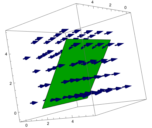
- In the pictures above, the velocity is given by $\vec F = (0,2,0)$ meters per second and the green surface $S$ is a square with surface area 25 square meters. For each picture above, let's determine the flux of $\vec F$ across $S$.
- Explain why the flow rate of $\vec F$ through $S$ for the first image above is 50 cubic meters per second.
- Explain why the flow rate of $\vec F$ through $S$ for the second image above is 0 cubic meters per second.
- In the third image, the edges of the parallelogram are given by $\vec u = (5,0,0)$ and $\vec v = (0,3,4)$. Compute the flow rate of $\vec F$ through $S$.
In our computations above, we were not concerned about which direction the fluid flowed through the surface. In general, we'll keep track of which direction a fluid flows through a surface, and count flux as negative when the fluid flows the opposite direction. To do this, we pick a unit vector $\hat n$ to the surface, called an orientation of $S$, and decide flux is positive precisely when the vector component of $\vec F$ that is parallel to $\hat n$ is in the same direction as $\hat n$.
- In the third image above, a normal vector to the surface is $\vec u\times \vec v = (5,0,0)\times (0,3,4) = (0,20,-15)$, which means we can use $\hat n = \frac{\vec u\times \vec v}{|\vec u\times \vec v|} = \frac{1}{5}(0,4,-3)$ as an orientation for $S$. Show that the flux of $\vec F$ across $S$ with the orientation $\hat n$ is $ ( \vec F\cdot \hat n)( \text{Surface Area of $S$ } )$.
The computations above generalize rapidly to provide a method for computing the flux of a vector field $\vec F$ across a surface $S$ in the direction of $\hat n$. For a vector field $\vec F$ and surface $S$ with orientation $\hat n$, we have used $dS$ to represent small bits of surface area. This means a small amount of flux across $S$ is given by $d\text{Flux} = \vec F\cdot \hat n dS$. Summing these, and computing a limit provides the flux as $$\text{Flux}=\Phi = \iint_S \vec F\cdot \hat n dS.$$ Note that because $\hat n$ is a unit normal vector to $S$, then given a parametrization $\vec r(u,v)$ of $S$ for $(u,v)$ in some region $R$, we know $\hat n = \pm \frac{\vec r_u\times \vec r_v}{|\vec r_u\times \vec r_v|} $ while $dS = |\vec r_u\times \vec r_v|dudv$. This means we can simplify the flux integral above to $$\text{Flux}=\Phi = \iint_R \vec F \cdot (\pm\vec r_u\times \vec r_v)dudv,$$ where the $\pm$ sign must be determined based on the orientation of the surface.
- Let $\vec F = (x^2 + y, y - z, 3 x + 2 z)$ and $S$ be the surface parametrized by $\vec r(u,v) = (3 \cos v,u,3\sin v)$ for $1\leq u\leq 5$ and $0\leq v\leq 2\pi$. Let $\hat n$ be the unit normal to $S$ which points outwards, away from the $y$-axis. Compute the outward flux $\Phi$ of $\vec F$ across $S$. The steps below can serve as a guide.
- Compute $\vec r_u$ and $\vec r_v$.
- Compute a normal vector $\vec N = \vec r_u \times \vec r_v$, and decide if $\vec N$ points in the same, or opposite direction, as the orientation $\hat n$. This may require you to draw the surface to visually make that determination.
- Insert all the known values into $\iint_R \vec F\cdot (\pm\vec r_u\times \vec r_v)dudv$, making sure all variables have been written in terms of $u$ and $v$. Then use software to compute the integral. (I got $72\pi$.)
- Let $\vec F = (2 y z, x + 3 y, -z^2)$ and $S$ be the surface parametrized by $\vec r(u,v) = (u \cos v, u \sin v, 9 - u^2)$ for $0\leq u\leq 3$ and $0\leq v\leq 2\pi$. Compute the upward ($\hat n$ has positive $z$-component) flux $\Phi$ of $\vec F$ across $S$ in the direction of $\hat n$. The steps above are still the same guide. (I got $-243\pi/2$.)
Task 42.2
For a surface $S$ with parametrization $\vec r(u,v) = (x(u,v),y(u,v),z(u,v))$ for $(u,v)$ in some region $R$, we have shown that surface area is $$S = \iint_S dS = \iint_R |\vec r_u\times\vec r_v|dudv.$$ This means we can compute mass, average values, centroids, centers-of-mass, etc, in a manner similar to what we have already done.
- For a function $f$ defined at points on the surface, the average value is $$\bar f = \frac{\iint_S f dS}{\iint_S dS} = \frac{\iint_R f(u,v) |\vec r_u\times\vec r_v| dudv}{\iint_R |\vec r_u\times\vec r_v| dudv}.$$ Replacing $f$ with $x$, $y$, or $z$ obtains the corresponding coordinate of the centroid of the surface.
- Given a density $\delta$ at points on the surface, the mass of the surface is $$ m = \iint_S dm = \iint_S \delta dS = \iint_R \delta(u,v) |\vec r_u\times\vec r_v| dudv.$$ The center-of-mass is given by $(\bar x, \bar y, \bar z) = \frac{\iint_S (x,y,z) \delta dS}{\iint_S \delta dS}$ which we can write as $$\begin{align*} \bar x &= \frac{\iint_R x(u,v) \delta(u,v) |\vec r_u\times\vec r_v| dudv}{\iint_R \delta(u,v) |\vec r_u\times\vec r_v| dudv},\\ \bar y &= \frac{\iint_R y(u,v) \delta(u,v) |\vec r_u\times\vec r_v| dudv}{\iint_R \delta(u,v) |\vec r_u\times\vec r_v| dudv},\\ \bar z &= \frac{\iint_R z(u,v) \delta(u,v) |\vec r_u\times\vec r_v| dudv}{\iint_R \delta(u,v) |\vec r_u\times\vec r_v| dudv}. \end{align*}$$
Note that there are lots of things going on with each integral. Software will greatly reduce the amount of time needed to set up and compute these integrals. The commands that will be most useful are ParametricPlot3D[], D[], Cross[], Norm[], and Integrate[].
- Consider the surface $\vec r(u,v) = (3\cos v,3\sin v, u)$ for $1\leq u\leq 5$ and $0\leq v\leq \pi$. Start by drawing the surface. From your picture, state $\bar x$ and $\bar z$. Then set up and compute an integral formula that gives the $y$-coordinate of the centroid.
- A satellite dish lies along the parametric surface $\vec r(u,v) = (u^2, u\cos v, u\sin v)$ for $0\leq u\leq 2$ and $0\leq v\leq 2\pi$. Start by drawing the surface. The temperature at points on and near the dish is given by $T(x,y,z) = x+z$. Set up and compute an integral formula that gives the average temperature of the satellite dish.
- The top half of the surface $S$ of a donut (a torus) can be parametrized by $\vec r(u,v) = ((5 - 3 \cos u) \cos v, (5 - 3 \cos u) \sin v, 3 \sin u)$ for $0\leq u\leq \pi$ and $0\leq v\leq 2\pi$. Imagine that someone puts icing on the top of this donut (so creates a surface), but the thickness of the icing is more on the top of the donut than on the sides. While not a perfect way to model this situation, we could use $\delta = kz$ for some constant $k$ as a way to model the surface with varying density. Show that the center-of-mass of the surface $S$ with density function $\delta = kz$ is $(\bar x, \bar y, \bar z) = (0,0,\frac{3\pi}{4})$.
Task 42.3
We've seen all the new notation that we'll encounter for the rest of the semester. This task has us practice using the notation we've learned.
- Consider the vector field $\vec F = (x,x-z,y+z)$, the surface $S$ parametrized by $\vec r(u,v)=(u^2, u\cos v, u\sin v)$ for $0\leq u\leq 2$ and $0\leq v\leq 2\pi$, and the curve $C$ parametrized by $\vec r(t) = (4,2\cos t, 2\sin t)$ for $0\leq t\leq 2\pi$.
- Draw the surface $S$ and curve $C$. How are these two objects related?
- Compute $\vec N = \vec r_u\times \vec r_v$ and determine if $\vec N$ points inward toward the $x$-axis, or outwards away from the $x$-axis.
- Set up and compute the integral $\ds \int_C Mdx+Ndy+Pdz$, computing the work done by $\vec F$ along $C$.
- Set up and compute $\ds \iint_S \vec \nabla \times \vec F\cdot \hat n dS$, computing the flux of the curl of $\vec F$ across $S$ in the direction $\hat n$ outwards away from the $y$-axis.
- Consider the vector field $\vec F = (x,x-z,y+z)$, the solid domain $D$ that lies inside the sphere $x^2+y^2+z^2=25$, and the surface $S$ parametrized by $\vec r(u,v)=(5\sin v\cos u, 5 \sin v \sin u, 5 \cos v)$ for $0\leq u\leq 2\pi$ and $0\leq v\leq \pi$.
- Draw the surface $S$ and domain $D$. How are these two objects related?
- Compute $\vec N = \vec r_u\times \vec r_v$ and determine if $\vec N$ points inward toward the domain $D$ or outwards away from the domain $D$.
- Set up and compute $\ds \iint_S \vec F\cdot \hat n dS$ for $\hat n$ pointing outwards, away from the solid inside $S$. This computes the outward flux of $\vec F$ across $S$.
- Set up and compute $\ds \iiint_D \vec \nabla \cdot \vec F dV$, the triple integral of the divergence of $\vec F$ over the domain $D$.
Task 42.4
Pick some problems related to the topics we are discussing from the Text Book Practice page.
Day 42 - In class
Brain Gains (Rapid Recall, Jivin' Generation)

- Draw the surface $S$ with parametrization $\vec r(u,v) = (u, u\cos v, u\sin v)$ for $1\leq u\leq 3$ and $0\leq v\leq \pi$.
- Set up the surface integral that would give the surface area of $S$.
- Set up the surface integral formula that would give the $z$-coordinate of the centroid of the surface $S$.
- Set up the surface integral that gives the flux $\Phi = \iint_S \vec F\cdot \hat n dS$ of the vector field $\vec F(x,y,z) = (2x+y,-yz^2, 3z)$ across the surface $S$ in the direction that points away from the $x$-axis.
Solutions
The solutions are all coded using the Mathematica code below. Note that the vector $n$ has a positive $x$-component, which means that the vector points inward towards the $y$-axis. The negative sign in the code below is needed to correctly get the flux.
r = {u, u Cos[v], u Sin[v]}
ParametricPlot3D[r, {u, 1, 3}, {v, 0, Pi}]
n = Cross[D[r, u], D[r, v]] // Simplify
Integrate[Norm[n], {u, 1, 3}, {v, 0, Pi}]
Integrate[u Sin[v] Norm[n], {u, 1, 3}, {v, 0, Pi}]/Integrate[Norm[n], {u, 1, 3}, {v, 0, Pi}]
Integrate[{2 u + u Cos[v], -u Cos[v] (u Sin[v])^2, 3 u Sin[v]} . -n, {u, 1, 3}, {v, 0, Pi}]
Integrate[ReplaceAll[{2 x + y, -y z^2, 3 z} . -n, {x -> u, y -> u Cos[v], z -> u Sin[v]}], {u, 1, 3}, {v, 0, Pi} ]
Show[
 ParametricPlot3D[r, {u, 1, 3}, {v, 0, Pi}],
 VectorPlot3D[{2 x + y, -y z^2, 3 z}, {x, 1, 3}, {y, -3, 3}, {z, 0, 3}]
 ]
Group Problems
- Consider the surface $S$ parametrized by $\vec r(u,v) = (u\cos v, u\sin v, u^2)$ for $0\leq u\leq 2$ and $0\leq v\leq 2\pi$.
- Draw the surface.
- Compute $dS = \left|\dfrac{\partial \vec r}{\partial u}\times\dfrac{\partial \vec r}{\partial v}\right|dudv$.
- Set up an integral formula to compute the surface area of $S$.
- Set up an integral formula to compute $\bar z$ for this surface.
- We would like an orientation $\hat n$ for the surface that points away from the $z$-axis. Does $ \dfrac{\partial \vec r}{\partial u}\times\dfrac{\partial \vec r}{\partial v}$ point towards the $z$-axis, or away from the $z$-axis?
- Set up the surface integral that gives the flux of $\vec F = (3yz,-2x+y, z-2x)$ across the surface $S$ in the direction of $\hat n$. Then use software to compute the integral.
- Consider the parametric surface $\vec r(u,v) = (u, u\cos v,u\sin v)$ for $0\leq v\leq \pi$ and $0\leq u\leq 4$.
- Draw the surface.
- Compute $dS = \left|\dfrac{\partial \vec r}{\partial u}\times\dfrac{\partial \vec r}{\partial v}\right|dudv$.
- Set up an integral formula to compute $\bar x$ for this surface.
- Give an equation of the tangent plane to the surface at $(u,v) = (1,\pi/2)$.
Day 43 - Prep
There is no new prep. Work on 41.3 and 42.1-3.
|
Sun |
Mon |
Tue |
Wed |
Thu |
Fri |
Sat |