
- I-Learn, Class Pictures, Learning Targets, Text Book Practice
- Prep Tasks: Unit 1 - Motion, Unit 2 - Derivatives, Unit 3 - Integration, Unit 4 - Vector Calculus
We still have some tasks from Day 19 to finish discussing in class.
Day 19 - Prep
Task 19.1
In the first calculus books, there was no mention of the chain rule. This is because differentials were extremely common notation, and the chain rule, when working with differentials, is simply substitution. In this task, we'll develop some rules for how to compute derivatives when functions depend on other functions (so composite functions).
- Suppose that $f(x,y,z) = ax+by+cz$, and $x=mt$, $y=nt$, and $z = pt$, for some constants $a,b,c,m,n,p$. Compute the differentials $df$, $dx$, $dy$, and $dz$. Then use substitution to obtain the differential of $f$ in terms of $t$ and $dt$. Finish by stating $\frac{df}{dt}$.
- Suppose now that $g$ is a function of $x$ and $y$, but $x$ and $y$ are functions of $u$, $v$, and $w$. This means, by definition of the differential and partial derivatives, that $dg = g_xdx+g_ydy$, along with $dx = x_udu+x_vdv+x_wdw$ and $dy = y_udu+y_vdv+y_wdw$. Substitution gives $$\begin{align*} dg &= g_xdx+g_ydy\\ &= g_x(x_udu+x_vdv+x_wdw)+g_y(y_udu+y_vdv+y_wdw)\\ &= (?)du+(?)dv+ (?)dw. \end{align*}$$ Fill in the question marks above, and then use your answer to state the three partials $\dfrac{\partial g}{\partial u}$, $g_v$, and $D_w g$.
- Consider the function $h(x,y,z)$, where $x$, $y$, and $z$ are functions of $r$ and $\theta$. State the differentials of $h$, $x$, $y$, and $z$, and then use substitution to prove that $$\dfrac{\partial h}{\partial r} = \dfrac{\partial h}{\partial x}\dfrac{\partial x}{\partial r} +\dfrac{\partial h}{\partial y}\dfrac{\partial y}{\partial r} +\dfrac{\partial h}{\partial z}\dfrac{\partial z}{\partial r}.$$ Obtain a similar formula for $\dfrac{\partial h}{\partial \theta}$.
Feel free to ask me in class how this relates to matrix multiplication.
Task 19.2
Suppose a rover travels around the circle $g(x,y)=x^2+y^2=1$. The elevation of the surrounding terrain is $f(x,y) = x^2+y+4$. The plot below shows the rover's path (the constraint $g(x,y)=1$), placed on the same grid as a contour plot of the elevation (the function $f(x,y)$ we wish to optimize).
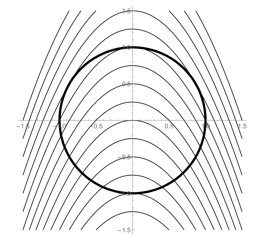
Each level curve above represents a difference in elevation of 0.25 m. Our goal is to find the maximum and minimum elevation reached by the rover as it travels around the circle. We will optimize $f(x,y)$ subject to the constraint $g(x,y)=1$.
- Label each level curve with its elevation. Print this page, or copy the curves down on your paper.
- At which $(x,y)$ point does the rover encounter the minimum elevation? What is the minimum elevation? Explain, using the plot.
- Suppose the rover is currently at the point $(0,1)$ on its circular path. As the rover moves left, will the elevation rise or fall? What if the rover moves right? Is $(0,1)$ the location of a local maximum or local minimum?
- On your graph, place a dot(s) where the rover reaches a maximum elevation. What is the maximum elevation? Explain.
- Rather than visually inspecting level curves, let's examine the gradients $\vec \nabla f$ and $\vec \nabla g$ to see how these gradients compare at maximums and minimums.
- On the graph above, draw $\vec \nabla f$ at lots of places on your contour plot.
- At lots of points on the circle, with a different color, draw $\vec \nabla g$.
- Make sure you draw both gradients at all the points corresponding to local maxes and mins.
- At the local maximums and minimums, Lagrange noticed that $\vec \nabla f = \lambda \vec \nabla g$.
- How would you interpret the equation $\vec \nabla f = \lambda \vec \nabla g$?
- Compute $\vec \nabla f$ and $\vec \nabla g$.
- Explain why the system of equations $\vec \nabla f = \lambda \vec \nabla g$ and $g(x,y)=c$ is equivalent to the system of equations $$2x = \lambda 2x,\quad 1=\lambda 2y,\quad x^2+y^2=1.$$
- Solve the system of equations above to obtain 4 ordered pairs $(x,y)$. You can use the Mathematica notebook LagrangeMultipliers.nb to check your work.
- At each ordered pair, find the elevation. What is the maximum elevation obtained, and where does it occur? What is the minimum elevation obtained, and where does it occur?
Suppose $f$ and $g$ are continuously differentiable functions. Suppose that we want to find the maximum and minimum values of $f(x,y)$ subject to the constraint $g(x,y)=c$ (where $c$ is some constant). If a local maximum or minimum occurs, it must occur at a spot where the gradient of $f$ and the gradient of $g$ point in the same, or opposite, directions. This means the gradient of $g$ must be a multiple of the gradient of $f$. To find the $(x,y)$ locations of the maximum and minimum values (if they exist), we solve the system of equations that result from $$\vec \nabla f = \lambda \vec \nabla g,\quad \text{and}\quad g(x,y)=c$$ where $\lambda$ is the proportionality constant. The locations of maximum and minimum values of $f$ will be among the solutions of this system of equations.
Task 19.3
This task will mostly involve reading through some definitions and an example, with a short example at the end.
Let $A$ be a square matrix, as $A=\begin{bmatrix} \begin{pmatrix}a\\b\end{pmatrix}& \begin{pmatrix}c\\d\end{pmatrix}\end{bmatrix} = \begin{bmatrix}a&c\\b&d\end{bmatrix}$. The eigenvalues $\lambda$ and eigenvectors $\vec x$ of $A$ are solutions $\lambda$ and $\vec x\neq \vec 0$ to the equation $A\vec x=\lambda \vec x$, effectively replacing the matrix product (linear combination) with scalar multiplication.
The identity matrix $I$ is a square matrix with 1's on the diagonal and zeros everywhere else, so in 2D we have $I = \begin{pmatrix} 1&0\\0&1 \end{pmatrix}$. To find the eigenvalues, we rewrite $A\vec x = \lambda\vec x$ in the form $A\vec x -\lambda\vec x=\vec 0$ or $A\vec x -\lambda I \vec x=\vec 0$, which becomes $(A-\lambda I) =\vec 0.$ We need to find the values $\lambda$ so that $\left(\begin{bmatrix} a&c\\b&d\end{bmatrix}-\lambda \begin{bmatrix} 1&0\\0&1 \end{bmatrix} \right)\begin{pmatrix}x\\y\end{pmatrix} =\begin{pmatrix}0\\0\end{pmatrix} \quad\text{or}\quad \begin{bmatrix} a-\lambda &c\\b&d-\lambda \end{bmatrix}\begin{pmatrix}x\\y\end{pmatrix} =\begin{pmatrix}0\\0\end{pmatrix}.$ A linear algebra course will show that $\lambda$ satisfies $$(a-\lambda)(d-\lambda)-bc=0.$$
Let $f(x,y)$ be a function so that all the second partial derivatives exist and are continuous. The second derivative of $f$, written $D^2f$ and sometimes called the Hessian of $f$, is a square matrix. Suppose $P=(a,b)$ is a critical point of $f$, meaning $\vec\nabla f(a,b) = (0,0)$.
- Suppose all the eigenvalues of $D^2f(a,b)$ are positive. Then at all points $(x,y)$ sufficiently near $P$, the gradient $\vec \nabla f(x,y)$ points away from $P$. The function has a local minimum at $P$.
- Suppose all the eigenvalues of $D^2f(a,b)$ are negative. Then at all points $(x,y)$ sufficiently near $P$, the gradient $\vec \nabla f(x,y)$ points inwards towards $P$. The function has a local maximum at $P$.
- Suppose the eigenvalues of $D^2f(a,b)$ differ in sign. Then at some points $(x,y)$ near $P$, the gradient $\vec \nabla f(x,y)$ points inwards towards $P$. However, at other points $(x,y)$ near $P$, the gradient $\vec \nabla f(x,y)$ points away from $P$. The function has a saddle point at $P$.
- If the largest or smallest eigenvalue of $f$ equals 0, then the second derivative tests yields no information.
Let's look at an example. Consider $f(x,y)=x^2-2x+xy+y^2$. The gradient is $\vec \nabla f(x,y)=(2x-2+y,x+2y)$. The critical points of $f$ occur where the gradient is zero. We need to solve the system $2x-2+y=0$ and $x+2y=0$, which is equivalent to solving $2x+y=2$ and $x+2y=0$. Double the second equation, and then subtract it from the first to obtain $0x-3y=2$, or $y=-2/3$. The second equation says that $x=-2y$, or that $x=4/3$. So the only critical point is $(4/3,-2/3)$.
The second derivatives is $ D^2f = \begin{bmatrix}2&1 \\1&2\end{bmatrix}.$ The second derivative is constant, so $D^2 f(4/3,-2/3)$ is the same as $D^2f(x,y)$. (In general, the critical point may affect your matrix.) To find the eigenvalues we solve $$(2-\lambda)(2-\lambda)-(1)(1)=0.$$ Expanding the left hand side gives $4-4\lambda + \lambda^2 -1 = 0$. Simplifying and factoring gives us $\lambda^2-4\lambda +3 = (\lambda-3)(\lambda -1) = 0$. The eigenvalues are $\lambda = 1$ and $\lambda=3$. Since both numbers are positive, we know the gradient points outwards away from the critical point. The critical point $(4/3,-2/3)$ corresponds to a local minimum of the function. The local minimum is the output $f(4/3,-2/3) = (4/3)^2-2(4/3)+(4/3)(-2/3)+(-2/3)^2$.
Let's try this process on our own. Consider the function $f(x,y)=x^2+4xy+y^2$.
- Find the critical points of $f$ by finding when $Df(x,y)$ is the zero matrix.
- Find the eigenvalues of $D^2f$ at any critical points.
- Label each critical point as a local maximum, local minimum, or saddle point, and state the value of $f$ at the critical point.
Task 19.4
Pick some problems related to the topics we are discussing from the Text Book Practice page.
Day 20 - Prep
Task 20.1
Consider the function $f(x,y)=x^3-3x+y^2-4y$.
- Find the critical points of $f$ by finding when $Df(x,y)$ is the zero matrix.
- Find the eigenvalues of $D^2f$ at any critical points. [Hint: First compute $D^2f$. Since there are two critical points, evaluate the second derivative at each point to obtain 2 different matrices. Then find the eigenvalues of each matrix.]
- Label each critical point as a local maximum, local minimum, or saddle point, and state the value of $f$ at the critical point.
- Use Mathematica to construct a 2D contour plot and 3D surface plot of the function to visually verify that your solution is correct. Choose bounds for your plots so that the critical points are clearly visible.
The Mathematica Notebook 2ndDerTest.nb can help you check much of your work above.
Task 20.2
Let's now return to a Lagrange multiplier problem, where we have a constraint that limits the values over which we want to optimize a function. Consider the curve $xy^2=54$.
- Start by drawing the curve.
The distance from each point on this curve to the origin is a function that must have a minimum value. We will find a point $(a,b)$ on the curve that is closest to the origin.
The first step to any Lagrange multiplier problem is to identify the function $f(x,y)$ that we wish to maximize or minimize, and then then identify the constraint and write it in the form $g(x,y) = c$. The distance from $(x,y)$ to the origin is $f(x,y) = \sqrt{(x-0)^2+(y-2)^2}=\sqrt{x^2+y^2}.$ This is the function we wish to minimize. The square root on this function will complicate computations later on. Because the square root function is increasing, note that $h(x,y) = x^2+y^2$ will have its minimum value at the same place. Because of this, we can simplify our work and use $f(x,y)=x^2+y^2$ as the function we wish to minimize.
- What's the constant $c$ and function $g$ so that our constraint can be written in the form $g(x,y)=c$?
- Solve the system $\vec \nabla f = \lambda \vec \nabla g$ and $g=c$.
- After computing the gradients, state the 3 equations that form the system we must solve, and then solve it.
- Note that in this problem, the number $\lambda$ is not an eigenvalue, rather it is a multiplier that helps us know if $\vec \nabla f$ and $\vec \nabla g$ lie on the same line (are parallel or antiparallel, i.e. "Is one gradient a multiple of the other?".
- State the $(x,y)$ coordinates on the curve $xy^2=54$ that are closest to the origin.
Remember that you can use LagrangeMultipliers.nb to check your work.
- How does the problem above change if we want to find the point on the curve that is closest to $(3,4)$? Solving the corresponding system of equations by hand will not be simple, but we can use the Mathematica notebook above to quickly answer this question, once we state $f$, $g$, and $c$. You will need to numerically approximate the solution that Mathematica gives (type //N at the end of a line of code to numerically approximate the output). The solution is $(x,y) = (3.11122,4.16612)$.
Task 20.3
Consider the function $f(x,y,z) = -x^2+y^2+z^2$.
- Start by using the ContourPlot3D[] command in Mathematica to draw several level surface of this function. You can use the Mathematica notebook ContourSurfaceGradient.nb to help you.
The level surface which passes through the point $(3,2,-1)$ is shown below, along with the tangent plane to the surface through the point $(3,2,-1)$. This surface is called a hyperboloid of two sheets.
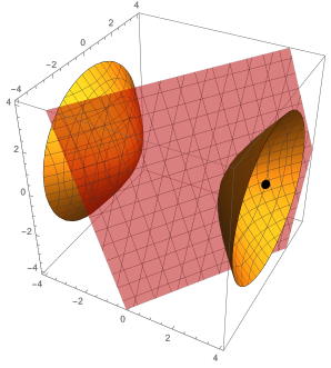
- Use the differential $$df = f_xdx+f_ydy+f_zdz \quad\text{or}\quad df=\vec\nabla f(a,b,c)\cdot(dx,dy,dz) . $$ to give an equation of the tangent plane to this surface at the point $(3,2,-1)$. [Hint: Start by explaining why $df=0$. Then we have $dx=x-3$, $dy=y-?$, and $dz =?$. Don't forget to evaluate the partials at the correct point.]
- Suppose the function $f(x,y,z) = -x^2+y^2+z^2$ gives the temperature (in Celcius) at points in space near some object (located at the origin), with $x,y,z$ values given in meters. Compute the temperature at $(3,2,-1)$, and then use differentials to approximate the temperature at $(3.01,1.98, -0.98)$. [What are $dx$, $dy$, and $dz$?]
- Compute the directional derivative of $f(x,y,z) = -x^2+y^2+z^2$ at the point $(3,2,-1)$ in the direction $(1, -2, 2)$. What are the units of $D_{ (1, -2, 2) }f(3,2,-1)$?
- What similarities, and what differences, do you see in the three questions above?
Task 20.4
Pick some problems related to the topics we are discussing from the Text Book Practice page.
Day 20 - In class
Brain Gains (Rapid Recall, Jivin' Generation)

- Consider the function $z=\sin(x)+e^y$, where $x=3t$ and $y=t^2$. Compute $\frac{dz}{dt}$.
Solution
There are two ways to do this.
- Substitution gives $z=\sin(3t)+e^{t^2}$. Differentiation (using the chain rule) then gives $$\frac{dz}{dt}=\cos(3t)\frac{d}{dt}(3t)+e^{t^2}\,\frac{d}{dt}(t^2)=\cos(3t)3+e^{t^2}\,2t.$$
- Differentials give $dz = \cos(x)dx+e^ydy$, with $dx = 3dt$ and $dy=2tdt$. Substitution then gives $$dz = \cos(3t)3dt+e^{t^2}\,2tdt\quad\text{or}\quad\frac{dz}{dt}=\cos(3t)3+e^{t^2}\,2t.$$
In both cases, we obtained the same solution of $$\frac{dz}{dt}=\underbrace{\cos(3t)}_{f_x}\underbrace{3}_{\frac{dx}{dt}}+\underbrace{e^{t^2}}_{f_y}\underbrace{2t}_{\frac{dy}{dt}}.$$ Writing the solution above symbolically gives us the chain rule $$\frac{dz}{dt} = f_x\frac{dx}{dt}+f_y\frac{dy}{dt} = \frac{\partial z}{\partial x}\frac{dx}{dt}+\frac{\partial z}{\partial y}\frac{dy}{dt}.$$
- Suppose $dz = e^{x^2}dx+\cos(2y)dy$, $x=3t$, and $y=t^2$. Compute $\frac{dz}{dt}$.
Solution
This time we don't know what the function $z$ equals, so we cannot first substitute and then differentiate. We do know however that $f_x = e^{x^2}$ and $f_y = \cos(2y)$. We can compute differentials and then substitute.
- Note that $dx = 3dt$ and $dy = 2tdt$. Substitution then gives $$dz = e^{(3t)^2}3\,dt+\cos(2(t^2))2t\,dt \quad\text{and so}\quad \frac{dz}{dt} = e^{(3t)^2}3+\cos(2(t^2))2t.$$
Again, the the solution above symbolically gives us the same chain rule $$\frac{dz}{dt} = f_x\frac{dx}{dt}+f_y\frac{dy}{dt} = \frac{\partial z}{\partial x}\frac{dx}{dt}+\frac{\partial z}{\partial y}\frac{dy}{dt}.$$
- For the function $f(x,y) = x^2y^4$, we have $\vec \nabla f(x,y) = (2xy^4,4x^2y^3)$. Compute the differential of $\vec \nabla f(x,y)$, and then state the second derivative $D^2f(x,y)$.
Solution
We have $$\begin{align} d(\vec\nabla f) &= d(2xy^4,4x^2y^3)\\ &= ((2dx)y^4+2x(4y^3dy),(8xdx)y^3+4x^2(3y^2dy))\\ &= \begin{pmatrix}(2)y^4\\(8x)y^3\end{pmatrix}dx+\begin{pmatrix}2x(4y^3)\\4x^2(3y^2)\end{pmatrix}dy\\ &= \begin{bmatrix}(2)y^4&2x(4y^3)\\(8x)y^3&4x^2(3y^2)\end{bmatrix}\begin{pmatrix}dx\\dy\end{pmatrix}. \end{align}$$ The last two lines above give the differential of $\vec \nabla f$ as a linear combination of partial derivatives, and then as a matrix product. The last line show the second derivative of $f$ is $$D^2f(x,y) = \begin{bmatrix}(2)y^4&2x(4y^3)\\(8x)y^3&4x^2(3y^2)\end{bmatrix} = \begin{bmatrix}2y^4&8xy^3\\8xy^3&12x^2y^2\end{bmatrix} .$$ We can also obtain this matrix by just directly computing all the second partial derivatives.
- $f_x = 2xy^4$ which means $f_{xx} = 2y^4$ and $f_{xy} = 8xy^3$. These form the first column.
- $f_y = 4x^2y^3$ which means $f_{yx} = 8xy^3$ and $f_{yy} = 12x^2y^2$. These form the second column.
Group Problems
- A rover travels along the line $g(x,y)=2x+3y=6$. The surrounding terrain has elevation $f(x,y)=x^2+4y$. The rover reaches a local minimum along this path, and our job is to find the location of this minimum.
- Compute $\vec \nabla f$ and $\vec \nabla g$.
- Write the system of equations that results from $\vec \nabla f=\lambda\vec \nabla g$ together with $g(x,y) = 6$.
- Solve the system above (you should get $x=4/3$ and $y=10/9$).
- Use LagrangeMultipliers.nb to check your work and visualize the rover's path and how it relates to the elevation contours. Scroll down to the "All Code in One Block" section, and update f, g, and c.
- For the function $f(x,y)=x^2+4xy+3y^2-10x-18y$, verify that the first derivative $Df(x,y)$ and second derivative $D^2f(x,y)$ are $$Df(x,y) = \begin{bmatrix}2x+4y-10&4x+6y-18\end{bmatrix}\quad\text{and}\quad
D^2f(x,y) = \begin{bmatrix}\begin{matrix}2\\4\end{matrix}&\begin{matrix}4\\6\end{matrix}\end{bmatrix}.
$$
- Solve $Df(x,y)=\begin{bmatrix}0&0\end{bmatrix}$, to find the critical points of this function. [Check: $(x,y)=(3,1)$.]
- Find the eigenvalues of $D^2f(3,1)$. [Check: $\lambda = 4\pm\sqrt{20} = 4\pm 2\sqrt{5}$.]
- Does the function $f$ have a local max, local min, or saddle at $(3,1)$? Explain.
- Consider the function $f(x,y,z) = 3xy+z^2$. We'll be analyzing the level surface that passes through the point $P=(1,-3,2)$.
- Compute the differential $df$, and then evaluate the differential at $P$.
- For a level surface, the output remains constant (so $df=0$). If we let $(x,y,z)$ be a point on the surface really close to $P$, then we have $dx=x-1$, $dy=y-(-3)$ and $dz = z-?$. Plug this information into the differential at $P$ to obtain an equation of the tangent plane.
- Give an equation of the tangent plane to the level surface of $f$ that passes through $(1,2,-3)$.
- Give an equation of the tangent plane to the level surface of $f$ that passes through $(a,b,c)$.
- What relationship exists between the gradient of $f$ at $P$ and the tangent plane through $P$?
- Suppose a plane passes through the point $(a,b,c)$ and has normal vector $(A,B,C)$. Give an equation of that plane.
- Give an equation of the tangent plane to $xy+z^2=7$ at the point $P=(-3,-2,1)$.
- Give an equation of the tangent plane to $z=f(x,y)=xy^2$ at the point $P=(4,-1,f(4,-1))$.
Day 21 - Prep
Task 21.1
Let $f(x,y) = 9-x^2-y^2$. Rather than using Cartesian coordinates to examine this function, we could instead use polar coordinates $x=r\cos \theta$ and $y=r\sin\theta$.
- Compute the differential $df$ in terms of $x$, $y$, $dx$, and $dy$.
- Compute the differentials $dx$ and $dy$ in terms of $r$, $\theta$, $dr$, and $d\theta$.
- Use substitution to obtain $df$ in terms of $r$, $\theta$, $dr$, and $d\theta$. Write your answer as the linear combination $df = (?)dr + (?)d\theta$.
- State $\frac{\partial f}{\partial r}$ and $\frac{\partial f}{\partial \theta}$.
- We can write the change of coordinates as the function $(x,y) = \vec T(r,\theta) = (r\cos\theta, r\sin\theta)$. Given a polar coordinate $(r,\theta)$, the function $\vec T$ returns the Cartesian (rectangular) coordinate $(x,y)$. Compute $f(\vec T(r,\theta))$.
- Compute the differential $d\vec T$ and write is as the linear combination $d\vec T = (?)dr + (?)d\theta$. Note that the questions marks will be vectors, not numbers, because the function $\vec T$ returns a vector (not a number).
- State the total derivatives $Df(x,y)$ and $D\vec T(r,\theta)$. How would you interpret $Df(\vec T(r,\theta))$.
- Compute the matrix product $Df(\vec T(r,\theta))D\vec T(r,\theta)$. [Hint: the partial derivatives you computed earlier should appear.]
Task 21.2
This task will have you practice using the second derivative test to locate maxima, minima, and/or saddle points for function $f(x,y)$ of two variables.
- Consider the function $f(x,y)=x^3-3x+y^2-4y$.
- Find the critical points of $f$ by finding when $Df(x,y)$ is the zero matrix.
- Find the eigenvalues of $D^2f$ at any critical points. [Hint: First compute $D^2f$. Since there are two critical points, evaluate the second derivative at each point to obtain 2 different matrices. Then find the eigenvalues of each matrix.]
- Label each critical point as a local maximum, local minimum, or saddle point, and state the value of $f$ at the critical point.
- Consider the function $f(x,y) = 6x^2-2x^3+3y^2+6xy$. The function has two critical points $(0,0)$ and $(1,-1)$. At each of these points, evaluate the second derivative and then find the corresponding eigenvalues. Use these eigenvalues to classify each critical point as the location of a local maximum, local minimum, or saddle point.
The Mathematica Notebook 2ndDerTest.nb can help you check much of your work above.
Task 21.3
To use Lagrange Multipliers, we must (1) identify the function $f(x,y)$ to be optimized along with the constant $c$ and function $g$ in the constraint $g(x,y)=c$, (2) write the system of equations that results from $\vec \nabla f = \lambda \vec \nabla g$ and $g(x,y)=c$, (3) solve this system, and (4) determine which points correspond to maxes and which to mins. The third step, solving a system of equations, can become extremely difficult quite quickly, but luckily modern software can help facilitate this part of the process. Please use the Mathematica notebook LagrangeMultipliers.nb to help you check your work and visual what you're doing in this task.
- Let $f(x,y) = 20 x + 2 y^2$. Use Lagrange multipliers to identify the location of any extreme values of $f$ along the line $100=4x+8y$. Complete this by hand, and then check your work with software.
- A rover travels along a circle of radius 5, centered at the origin. The elevation of the surrounding hill is give by $z = 4x^2-4xy+y^2$. What are the highest and lowest elevations reached by the rover? [If the system to solve is brutal, then use software to help you.]
Task 21.4
Pick some problems related to the topics we are discussing from the Text Book Practice page.
|
Sun |
Mon |
Tue |
Wed |
Thu |
Fri |
Sat |